


This post introduces neural programs: the composition of neural networks with general programs, such as those written in a traditional programming language or an API call to an LLM. We present new neural programming tasks that consist of generic Python and calls to GPT-4. To learn neural programs, we develop ISED, an algorithm for data-efficient learning of neural programs.
Neural programs are the composition of a neural model $M_\theta$ followed by a program $P$. Neural programs can be used to solve computational tasks that neural perception alone cannot solve, such as those involving complex symbolic reasoning.
Neural programs also offer the opportunity to interface existing black-box programs, such as GPT or other custom software, with the real world via sensoring/perception-based neural networks. $P$ can take many forms, including a Python program, a logic program, or a call to a state-of-the-art foundation model. One task that can be expressed as a neural program is scene recognition, where $M_\theta$ classifies objects in an image and $P$ prompts GPT-4 to identify the room type given these objects.
Click on the thumbnails to see different examples of neural programs:

-
Neural Program for Scene Recognition 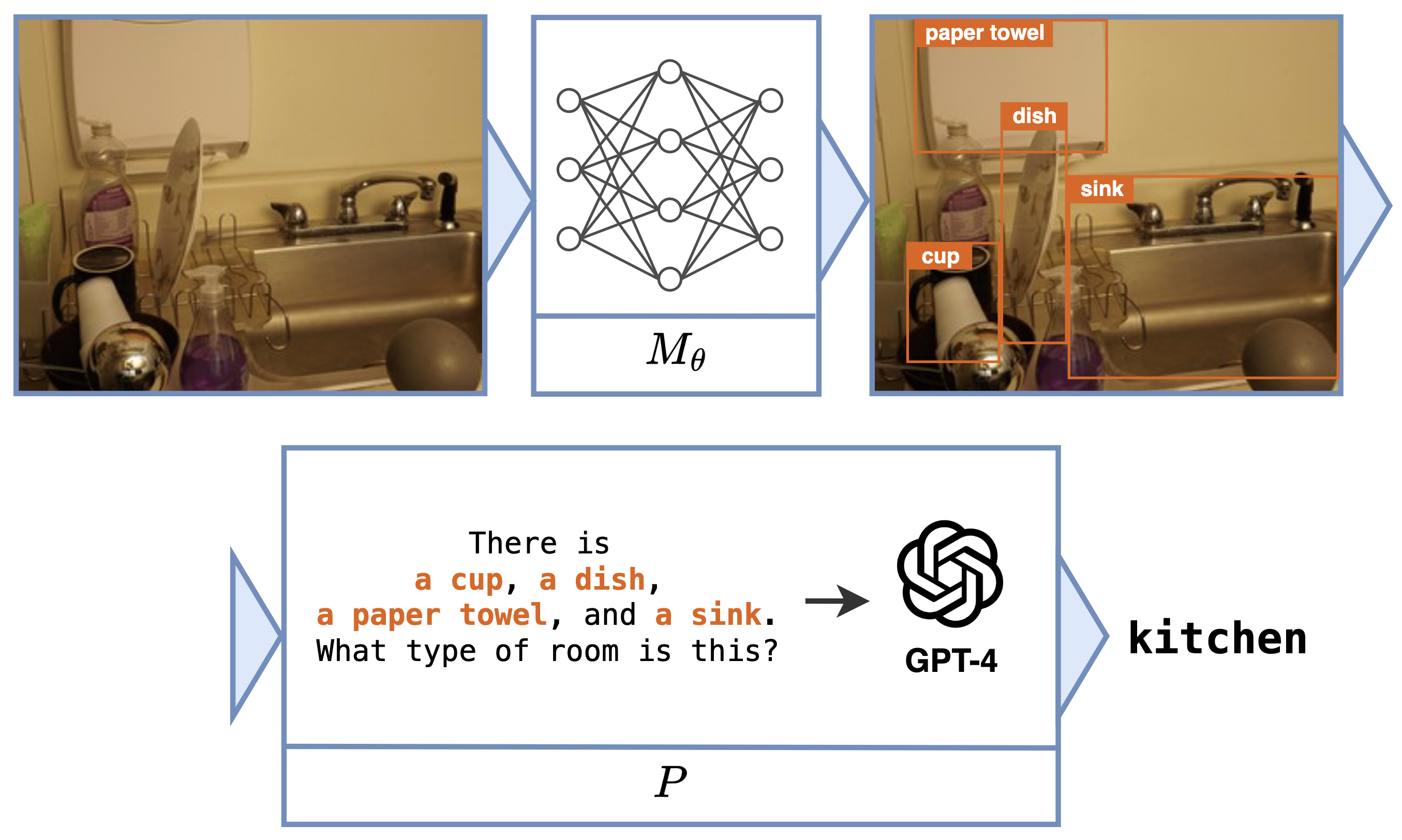
-
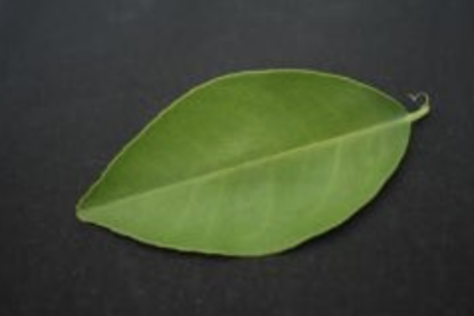
Neural Program for Leaf Classification 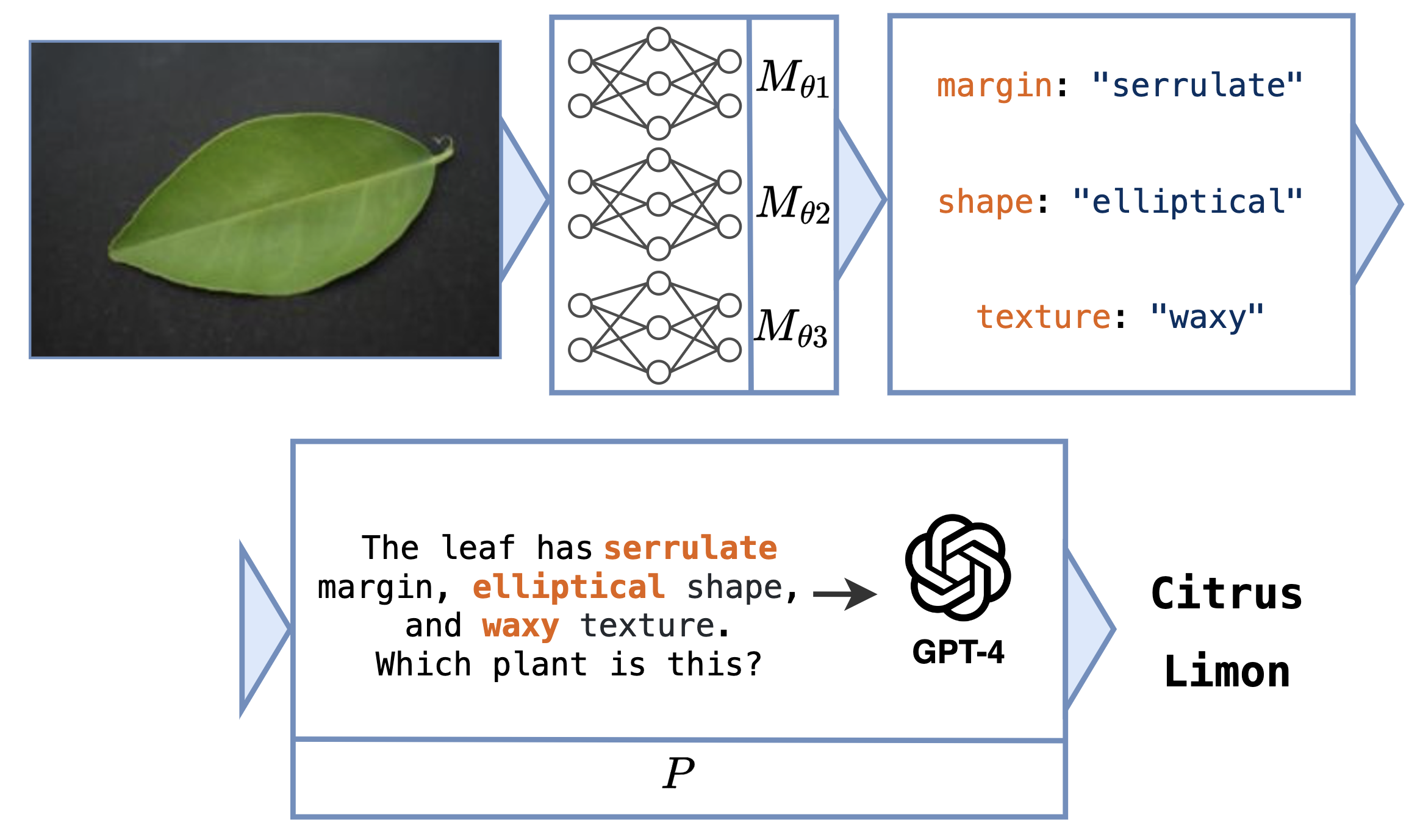
-
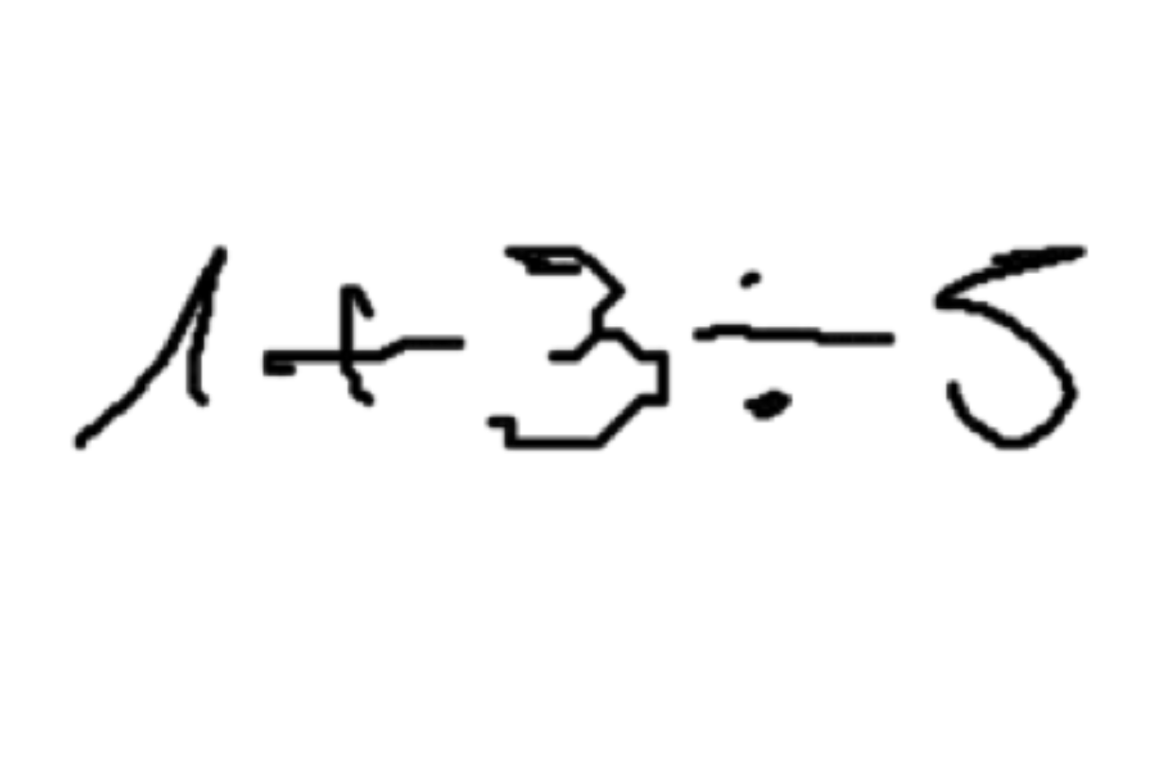
Neural Program for Hand-Written Formula 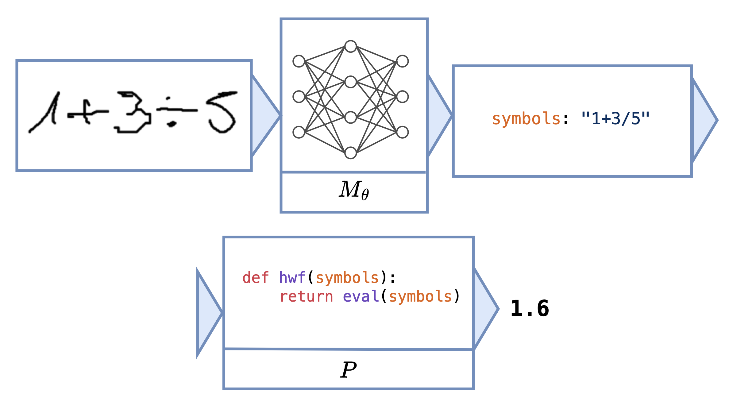
-
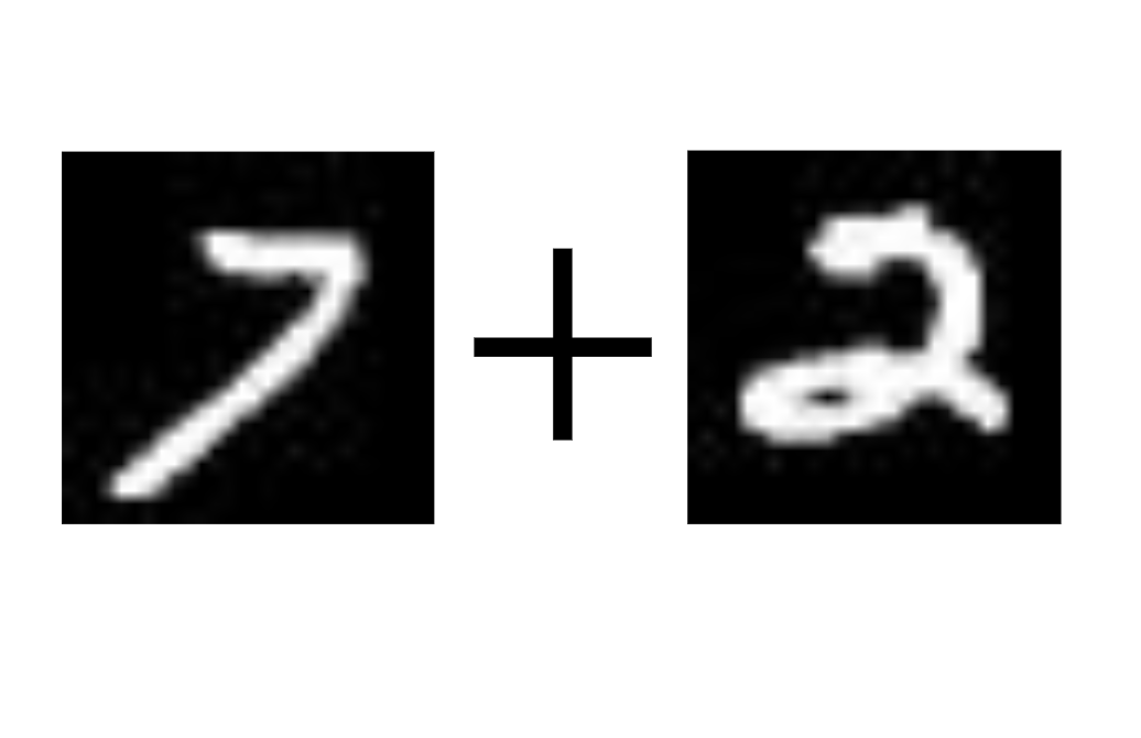
Neural Program for 2-Digit Addition 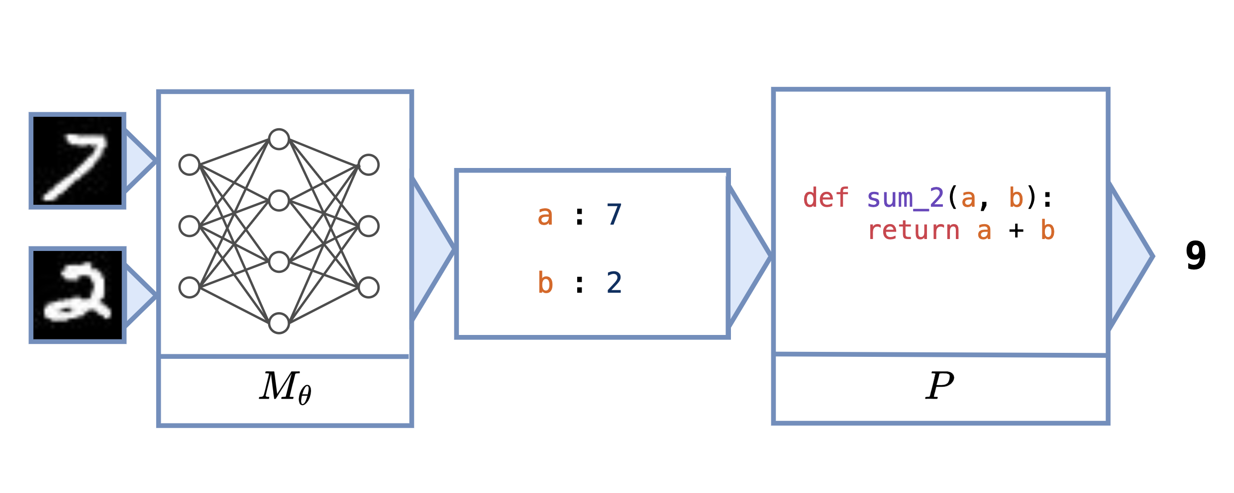
-
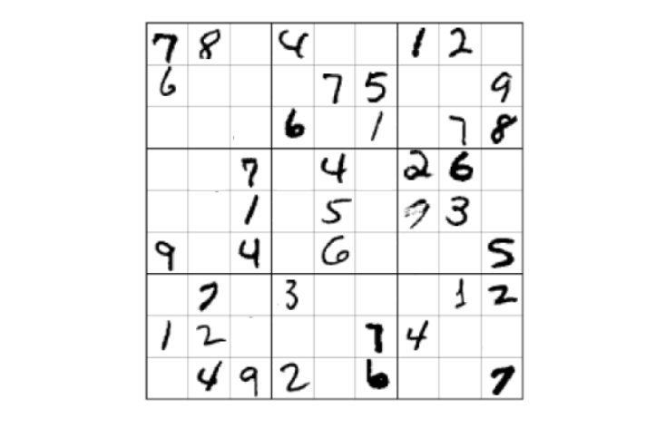
Neural Program for Sudoku Solving 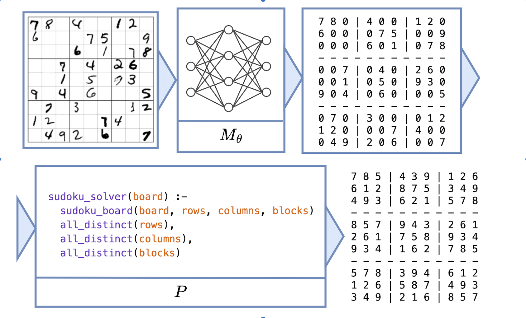
These tasks can be difficult to learn without intermediate labels for training $M_\theta$. The main challenge concerns how to estimate the gradient across $P$ to facilitate end-to-end learning.
Neurosymbolic Learning Frameworks
Neurosymbolic learning is one instance of neural program learning in which $P$ is a logic program. Scallop and DeepProbLog (DPL) are neurosymbolic learning frameworks that use Datalog and ProbLog respectively.
Click on the thumbnails to see examples of neural programs expressed as logic programs in Scallop.
Notice how some programs are much more verbose than they would be if written in Python.
For instance, the Python program for Hand-Written Formula could be a single line of code calling the built-in eval function,
instead of the manually built lexer, parser, and interpreter.
-
Scallop Program for Leaf Classification using a Decision Tree rel label = {("Alstonia Scholaris",),("Citrus limon",), ("Jatropha curcas",),("Mangifera indica",), ("Ocimum basilicum",),("Platanus orientalis",), ("Pongamia Pinnata",),("Psidium guajava",), ("Punica granatum",),("Syzygium cumini",), ("Terminalia Arjuna",)} rel leaf(m,s,t) = margin(m), shape(s), texture(t) rel predict_leaf("Ocimum basilicum") = leaf(m, _, _), m == "serrate" rel predict_leaf("Jatropha curcas") = leaf(m, _, _), m == "indented" rel predict_leaf("Platanus orientalis") = leaf(m, _, _), m == "lobed" rel predict_leaf("Citrus limon") = leaf(m, _, _), m == "serrulate" rel predict_leaf("Pongamia Pinnata") = leaf("entire", s, _), s == "ovate" rel predict_leaf("Mangifera indica") = leaf("entire", s, _), s== "lanceolate" rel predict_leaf("Syzygium cumini") = leaf("entire", s, _), s == "oblong" rel predict_leaf("Psidium guajava") = leaf("entire", s, _), s == "obovate" rel predict_leaf("Alstonia Scholaris") = leaf("entire", "elliptical", t), t == "leathery" rel predict_leaf("Terminalia Arjuna") = leaf("entire", "elliptical", t), t == "rough" rel predict_leaf("Citrus limon") = leaf("entire", "elliptical", t), t == "glossy" rel predict_leaf("Punica granatum") = leaf("entire", "elliptical", t), t == "smooth" rel predict_leaf("Terminalia Arjuna") = leaf("undulate", s, _), s == "elliptical" rel predict_leaf("Mangifera indica") = leaf("undulate", s, _), s == "lanceolate" rel predict_leaf("Syzygium cumini") = leaf("undulate", s, _) and s != "lanceolate" and s != "elliptical" rel get_prediction(l) = label(l), predict_leaf(l) -
Scallop Program for Hand-Written Formula // Inputs type symbol(u64, String) type length(u64) // Facts for lexing rel digit = {("0", 0.0), ("1", 1.0), ("2", 2.0), ("3", 3.0), ("4", 4.0), ("5", 5.0), ("6", 6.0),("7", 7.0), ("8", 8.0), ("9", 9.0)} rel mult_div = {"*", "/"} rel plus_minus = {"+", "-"} // Symbol ID for node index calculation rel symbol_id = {("+", 1), ("-", 2), ("*", 3), ("/", 4)} // Node ID Hashing @demand("bbbbf") rel node_id_hash(x, s, l, r, x + sid * n + l * 4 * n + r * 4 * n * n) = symbol_id(s, sid), length(n) // Parsing rel value_node(x, v) = symbol(x, d), digit(d, v), length(n), x < n rel mult_div_node(x, "v", x, x, x, x, x) = value_node(x, _) rel mult_div_node(h, s, x, l, end, begin, end) = symbol(x, s), mult_div(s), node_id_hash(x, s, l, end, h), mult_div_node(l, _, _, _, _, begin, x - 1), value_node(end, _), end == x + 1 rel plus_minus_node(x, t, i, l, r, begin, end) = mult_div_node(x, t, i, l, r, begin, end) rel plus_minus_node(h, s, x, l, r, begin, end) = symbol(x, s), plus_minus(s), node_id_hash(x, s, l, r, h), plus_minus_node(l, _, _, _, _, begin, x - 1), mult_div_node(r, _, _, _, _, x + 1, end) // Evaluate AST rel eval(x, y, x, x) = value_node(x, y) rel eval(x, y1 + y2, b, e) = plus_minus_node(x, "+", i, l, r, b, e), eval(l, y1, b, i - 1), eval(r, y2, i + 1, e) rel eval(x, y1 - y2, b, e) = plus_minus_node(x, "-", i, l, r, b, e), eval(l, y1, b, i - 1), eval(r, y2, i + 1, e) rel eval(x, y1 * y2, b, e) = mult_div_node(x, "*", i, l, r, b, e), eval(l, y1, b, i - 1), eval(r, y2, i + 1, e) rel eval(x, y1 / y2, b, e) = mult_div_node(x, "/", i, l, r, b, e), eval(l, y1, b, i - 1), eval(r, y2, i + 1, e), y2 != 0.0 // Compute result rel result(y) = eval(e, y, 0, n - 1), length(n) -
Scallop Program for 2-Digit Addition rel digit_1 = {(0,),(1,),(2,),(3,),(4,),(5,),(6,),(7,),(8,),(9,)} rel digit_2 = {(0,),(1,),(2,),(3,),(4,),(5,),(6,),(7,),(8,),(9,)} rel sum_2(a + b) :- digit_1(a), digit_2(b)
When $P$ is a logic program, techniques have been developed for differentiation by exploiting its structure. However, these frameworks use specialized languages that offer a narrow range of features. The scene recognition task, as described above, can’t be encoded in Scallop or DPL due to its use of GPT-4, which cannot be expressed as a logic program.
To solve the general problem of learning neural programs, a learning algorithm that treats $P$ as black-box is required. By this, we mean that the learning algorithm must perform gradient estimation through $P$ without being able to explicitly differentiate it. Such a learning algorithm must rely only on symbol-output pairs that represent inputs and outputs of $P$.
Black-Box Gradient Estimation
Previous works on black-box gradient estimation can be used for learning neural programs. REINFORCE samples from the probability distribution output by $M_\theta$ and computes the reward for each sample. It then updates the parameter to maximize the log probability of the sampled symbols weighed by the reward value.
There are different variants of REINFORCE, including IndeCateR that improves upon the sampling strategy to lower the variance of gradient estimation and NASR that targets efficient finetuning with single sample and custom reward function. A-NeSI instead uses the samples to train a surrogate neural network of $P$, and updates the parameter by back-propagating through this surrogate model.
While these techniques can achieve high performance on tasks like Sudoku solving and MNIST addition, they struggle with data inefficiency (i.e., learning slowly when there are limited training data) and sample inefficiency (i.e., requiring a large number of samples to achieve high accuracy).
Our Approach: ISED
Now that we understand neurosymbolic frameworks and algorithms that perform black-box gradient estimation, we are ready to introduce an algorithm that combines concepts from both techniques to facilitate learning.
Suppose we want to learn the task of adding two MNIST digits (sum$_2$). In Scallop, we can express this task with the program
sum_2(a + b) :- digit_1(a), digit_2(b)
and Scallop allows us to differentiate across this program. In the general neural program learning setting, we don’t assume that we can differentiate $P$, and we use a Python program for evaluation:
    def sum_2(a, b):
        return a + b
We introduce Infer-Sample-Estimate-Descend (ISED), an algorithm that produces a summary logic program representing the task using only forward evaluation, and differentiates across the summary. We describe each step of the algorithm below.
Step 1: Infer
The first step of ISED is for the neural models to perform inference. In this example, $M_\theta$ predicts distributions for digits $a$ and $b$. Suppose that we obtain the following distributions:
$p_b = [p_{b0}, p_{b1}, p_{b2}] = [0.2, 0.1, 0.7]$
Step 2: Sample
ISED is initialized with a sample count $k$, representing the number of samples to take from the predicted distributions in each training iteration.
Suppose that we initialize $k=3$, and we use a categorical sampling procedure. ISED might sample the following pairs of symbols: (1, 2), (1, 0), (2, 1). ISED would then evaluate $P$ on these symbol pairs, obtaining the outputs 3, 1, and 3.
Step 3: Estimate
ISED then takes the symbol-output pairs obtained in the last step and produces the following summary logic program:
    a = 1 /\ b = 2 -> y = 3
    a = 1 /\ b = 0 -> y = 1
    a = 2 /\ b = 1 -> y = 3
ISED differentiates through this summary program by aggregating the probabilities of inputs for each possible output.
In this example, there are 5 possible output values (0-4). For $y=3$, ISED would consider the pairs (1, 2) and (2, 1) in its probability aggregation. This resulting aggregation would be equal to $p_{a1} * p_{b2} + p_{a2} * p_{b1}$. Similarly, the aggregation for $y=1$ would consider the pair (1, 0) and would be equal to $p_{a1} * p_{b0}$.
We say that this method of aggregation uses the add-mult semiring, but a different method of aggregation called the min-max semiring uses min instead of mult and max instead of add. Different semirings might be more or less ideal depending on the task.
We restate the predicted distributions from the neural model and show the resulting prediction vector after aggregation. Hover over the elements to see where they originated from in the predicted distributions.
$p_a = \left[ \right. $$0.1$$, $ $0.6$$, $ $0.3$$\left. \right]$
$p_b = \left[ \right. $$0.2$$, $ $0.1$$, $ $0.7$$\left. \right]$
⎢
⎢
⎢
⎣
⎥
⎥
⎥
⎦
We then set $\mathcal{l}$ to be equal to the loss of this prediction vector and a one-hot vector representing the ground truth final output.
Step 4: Descend
The last step is to optimize $\theta$ based on $\frac{\partial \mathcal{l}}{\partial \theta}$ using a stochastic optimizer (e.g., Adam optimizer). This completes the training pipeline for one example, and the algorithm returns the final $\theta$ after iterating through the entire dataset.
Summary
We provide an interactive explanation of the differences between the different methods discussed in this blog post. Click through the different methods to see the differences in how they differentiate across programs. You can also sample different values for ISED and REINFORCE and change the semiring used in Scallop.
Ground truth: $a = 1$, $b = 2$, $y = 3$.
Assume $ M_\theta(a) = $ and $ M_\theta(b) = $ .

Evaluation
We evaluate ISED on 16 tasks. Two tasks involve calls to GPT-4 and therefore cannot be specified in neurosymbolic frameworks. We use the tasks of scene recognition, leaf classification (using decision trees or GPT-4), Sudoku solving, Hand-Written Formula (HWF), and 11 other tasks involving operations over MNIST digits (called MNIST-R benchmarks).
Our results demonstrate that on tasks that can be specified as logic programs, ISED achieves similar, and sometimes superior accuracy compared to neurosymbolic baselines. Additionally, ISED often achieves superior accuracy compared to black-box gradient estimation baselines, especially on tasks in which the black-box component involves complex reasoning. Our results demonstrate that ISED is often more data- and sample-efficient than state-of-the-art baselines.
Performance and Accuracy
Our results show that ISED achieves comparable, and often superior accuracy compared to neurosymbolic and black-box gradient estimation baselines on the benchmark tasks.
We use Scallop, DPL, REINFORCE, IndeCateR, NASR, and A-NeSI as baselines. We present our results in the tables below, divided by “custom” tasks (HWF, leaf, scene, and sudoku), MNIST-R arithmetic, and MNIST-R other. “N/A” indicates that the task cannot be programmed in the given framework, and “TO” means that there was a timeout.
| HWF | DT leaf | GPT leaf | scene | sudoku | |
|---|---|---|---|---|---|
| DPL | TO | 81.13 | N/A | N/A | TO |
| Scallop | 96.65 | 81.13 | N/A | N/A | TO |
| A-NeSI | 3.13 | 78.82 | 72.40 | 61.46 | 26.36 |
| REINFORCE | 88.27 | 40.24 | 53.84 | 12.17 | 79.08 |
| IndeCateR | 95.08 | 78.71 | 69.16 | 12.72 | 66.50 |
| NASR | 1.85 | 16.41 | 17.32 | 2.02 | 82.78 |
| ISED | 97.34 | 82.32 | 79.95 | 68.59 | 80.32 |
Despite treating $P$ as a black-box, ISED outperforms neurosymbolic solutions on many tasks. In particular, while neurosymbolic solutions time out on Sudoku, ISED achieves high accuracy and even comes within 2.46% of NASR, the state-of-the art solution for this task.
The baseline that comes closest to ISED on most tasks is A-NeSI. However, since A-NeSI trains a neural model to approximate the program and its gradient, it struggles to learn tasks involving complex programs, namely HWF and Sudoku.
Data Efficiency
We demonstrate that when there are limited training data, ISED learns faster than A-NeSI, a state-of-the-art black-box gradient estimation baseline.
We compared ISED to A-NeSI in terms of data efficiency by evaluating them on the sum$_4$ task. This task involves just 5K training examples, which is less than what A-NeSI would have used in its evaluation on the same task (15K). In this setting, ISED reaches high accuracy much faster than A-NeSI, suggesting that it offers better data efficiency than the baseline.
Sample Efficiency
Our results suggest that on tasks with a large input space, ISED achieves superior accuracy compared to REINFORCE-based methods when we limit the sample count.
We compared ISED to REINFORCE, IndeCateR, and IndeCateR+, a variant of IndeCateR customized for higher dimensional settings, to assess how they compare in terms of sample efficiency. We use the task of MNIST addition over 8, 12, and 16 digits, while varying the number of samples taken. We report the results below.
| sum$_8$ | sum$_{12}$ | sum$_{16}$ | ||||
|---|---|---|---|---|---|---|
| $k=80$ | $k=800$ | $k=120$ | $k=1200$ | $k=160$ | $k=1600$ | |
| REINFORCE | 8.32 | 8.28 | 7.52 | 8.20 | 5.12 | 6.28 |
| IndeCateR | 5.36 | 89.60 | 4.60 | 77.88 | 1.24 | 5.16 |
| IndeCateR+ | 10.20 | 88.60 | 6.84 | 86.92 | 4.24 | 83.52 |
| ISED | 87.28 | 87.72 | 85.72 | 86.72 | 6.48 | 8.13 |
For lower numbers of samples, ISED outperforms all other methods on the three tasks, outperforming IndeCateR by over 80% on 8- and 12-digit addition. These results demonstrate that ISED is more sample efficient than than the baselines for these tasks. This is due to ISED providing a stronger learning signal than other REINFORCE-based methods. IndeCateR+ significantly outperforms ISED for 16-digit addition with 1600 samples, which suggests that our approach is limited in its scalability.
Limitations and Future Work
The main limitation of ISED concerns scaling with the dimensionality of the space of inputs to the program. For future work, we are interested in exploring better sampling techniques to allow for scaling to higher-dimensional input spaces. For example, techniques can be borrowed from the field of Bayesian optimization where such large spaces have traditionally been studied.
Another limitation of ISED involves its restriction of the structure of neural programs, only allowing the composition of a neural model followed by a program. Other types of composites might be of interest for certain tasks, such as a neural model, followed by a program, followed by another neural model. Improving ISED to be compatible with such composites would require a more general gradient estimation technique for the black-box components.
Conclusion
We proposed ISED, a data- and sample-efficient algorithm for learning neural programs. Unlike existing neurosymbolic frameworks which require differentiable logic programs, ISED is compatible with Python programs and API calls to GPT. We demonstrate that ISED achieves similar, and often better, accuracy compared to the baselines. ISED also learns in a more data- and sample-efficient manner compared to the baselines.
For more details about our method and experiments, see our paper and code.
Citation
@article{solkobreslin2024neuralprograms,
  title={Data-Efficient Learning with Neural Programs},
  author={Solko-Breslin, Alaia and Choi, Seewon and Li, Ziyang and Velingker, Neelay and Alur, Rajeev and Naik, Mayur and Wong, Eric},
  journal={arXiv preprint arXiv:2406.06246},
  year={2024}
}