Sum-of-Parts Models: Faithful Attributions for Groups of Features

We identify a fundamental barrier for feature attributions in faithfulness tests. To overcome this limitation, we create faithful attributions to groups of features. The groups from our approach help cosmologists discover knowledge about dark matter and galaxy formation.

ML models can assist physicians in diagnosing a variety of lung, heart, and other chest conditions from X-ray images. However, physicians only trust the decision of the model if an explanation is given and make sense to them. One form of explanation identifies regions of the X-ray. This identification of input features relevant to the prediction is called feature attribution.

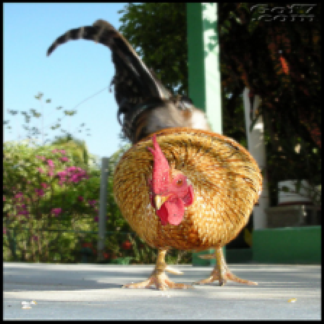
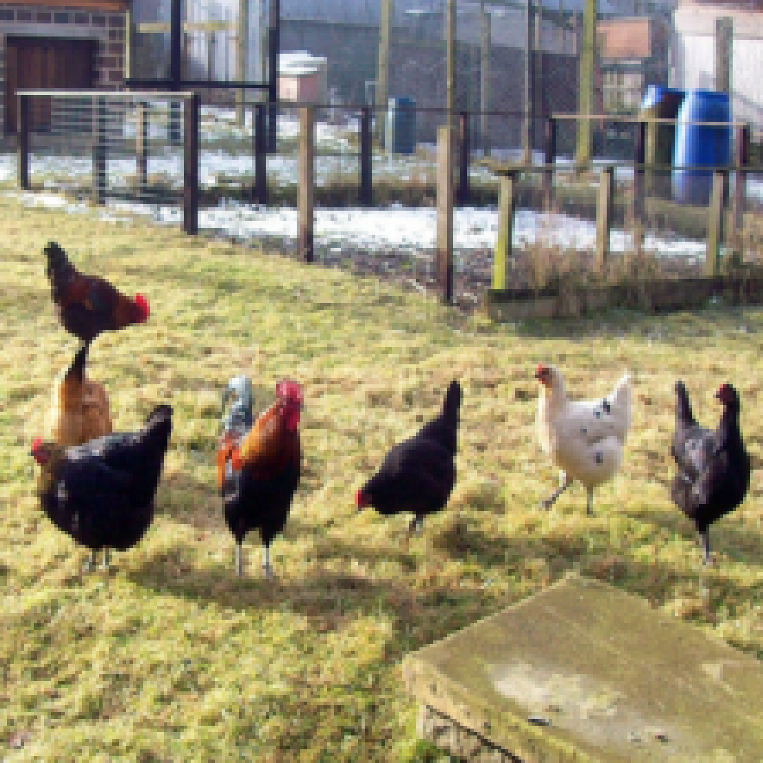
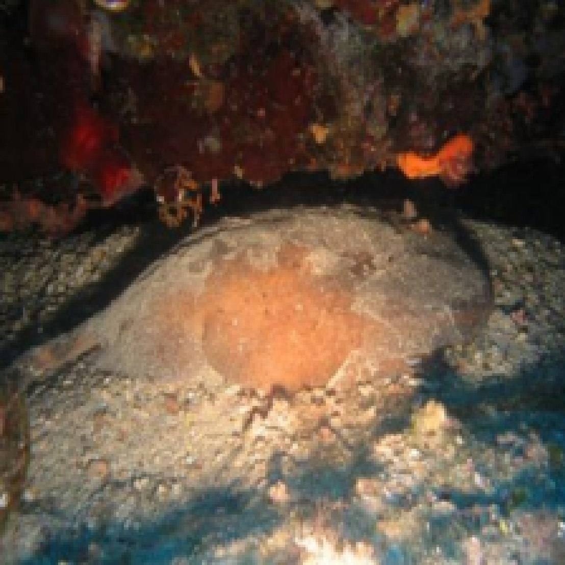
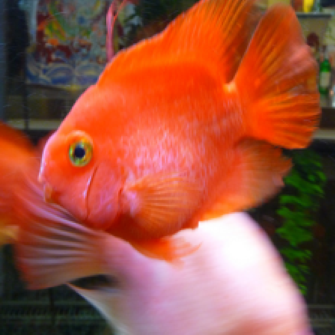
Click on the thumbnails to see different examples of feature attributions:

• 
• 
• 
• 
• 
• 
• 
• 
• 
• 

• LIME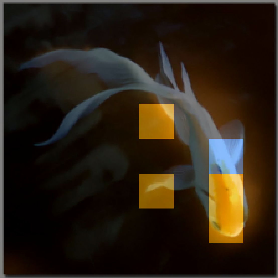

  

  SHAP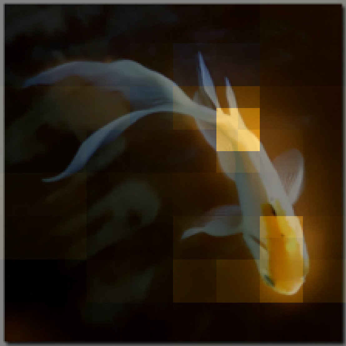

  

  RISE

  

  Grad-CAM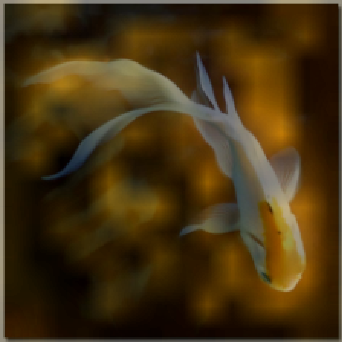

  

  IntGrad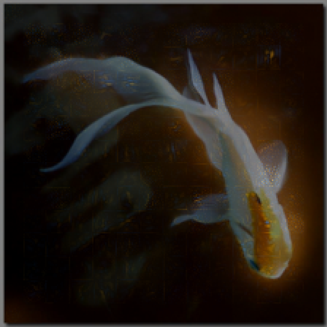

  

  FRESH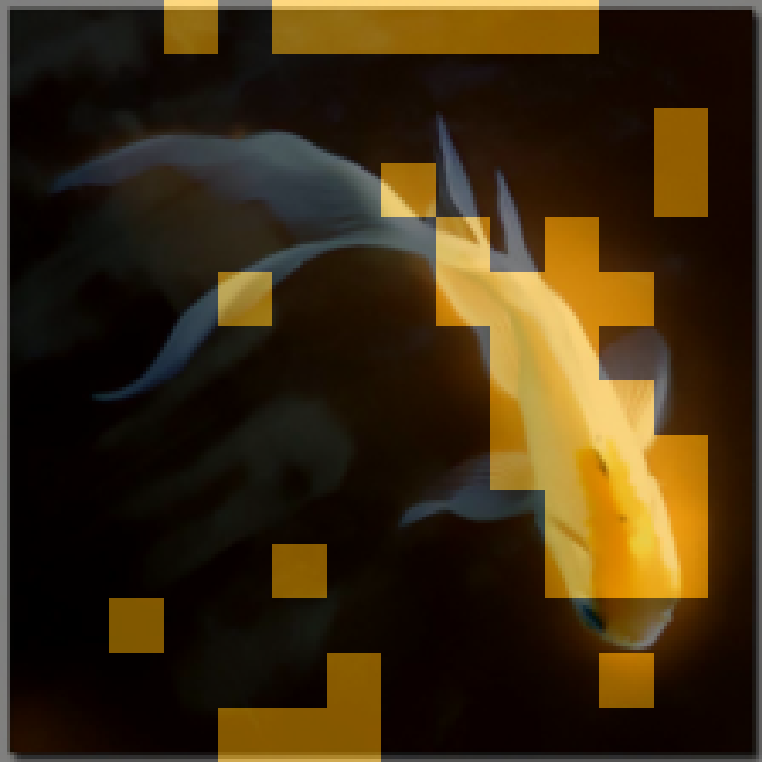

  

• LIME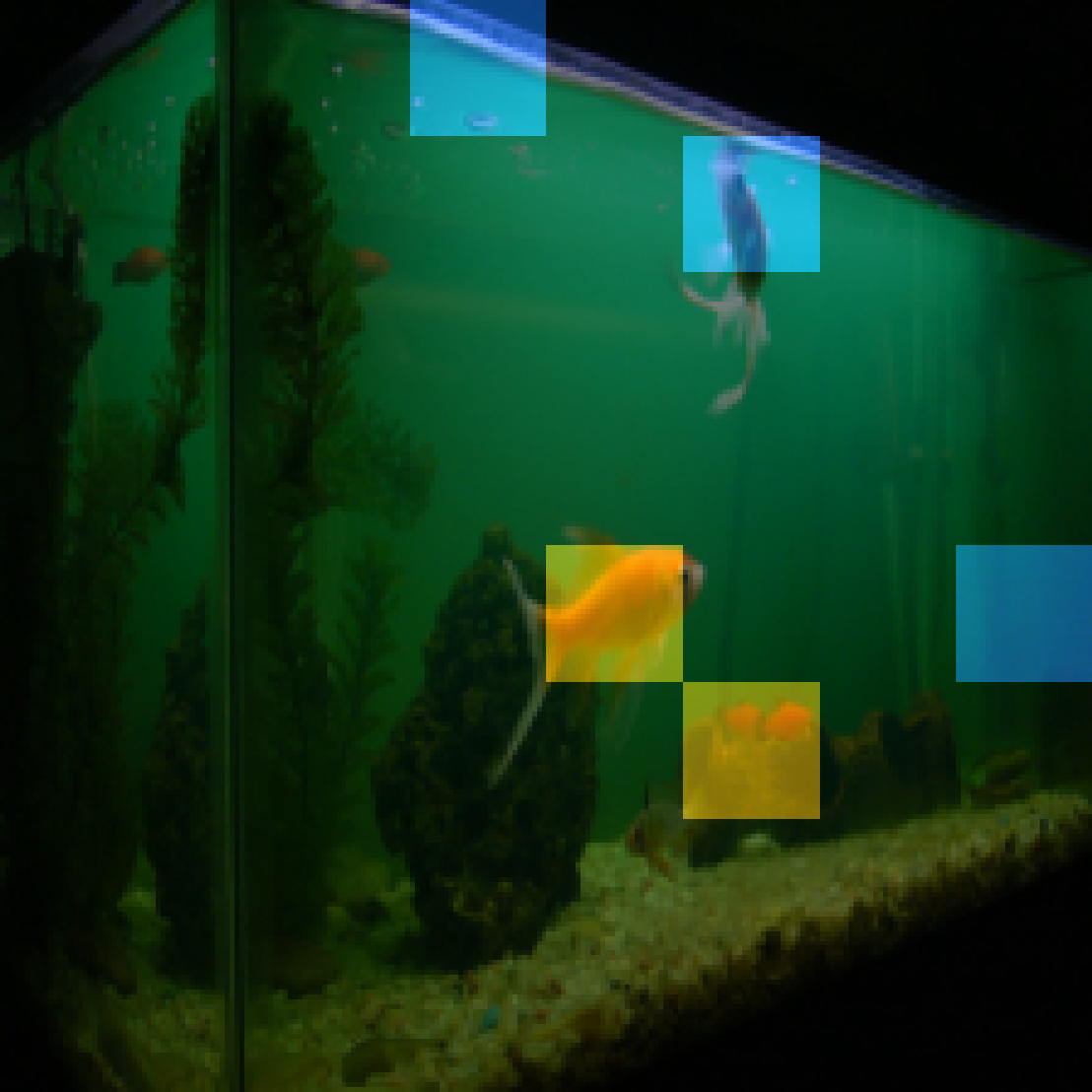

  

  SHAP

  

  RISE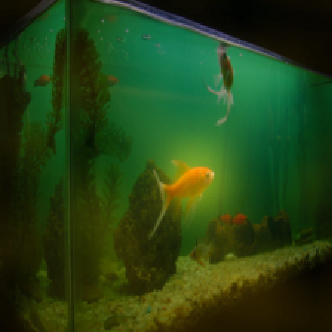

  

  Grad-CAM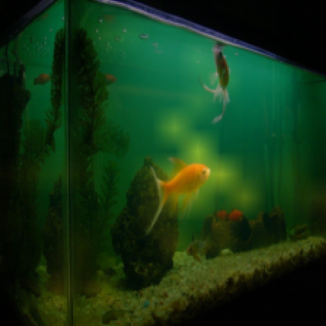

  

  IntGrad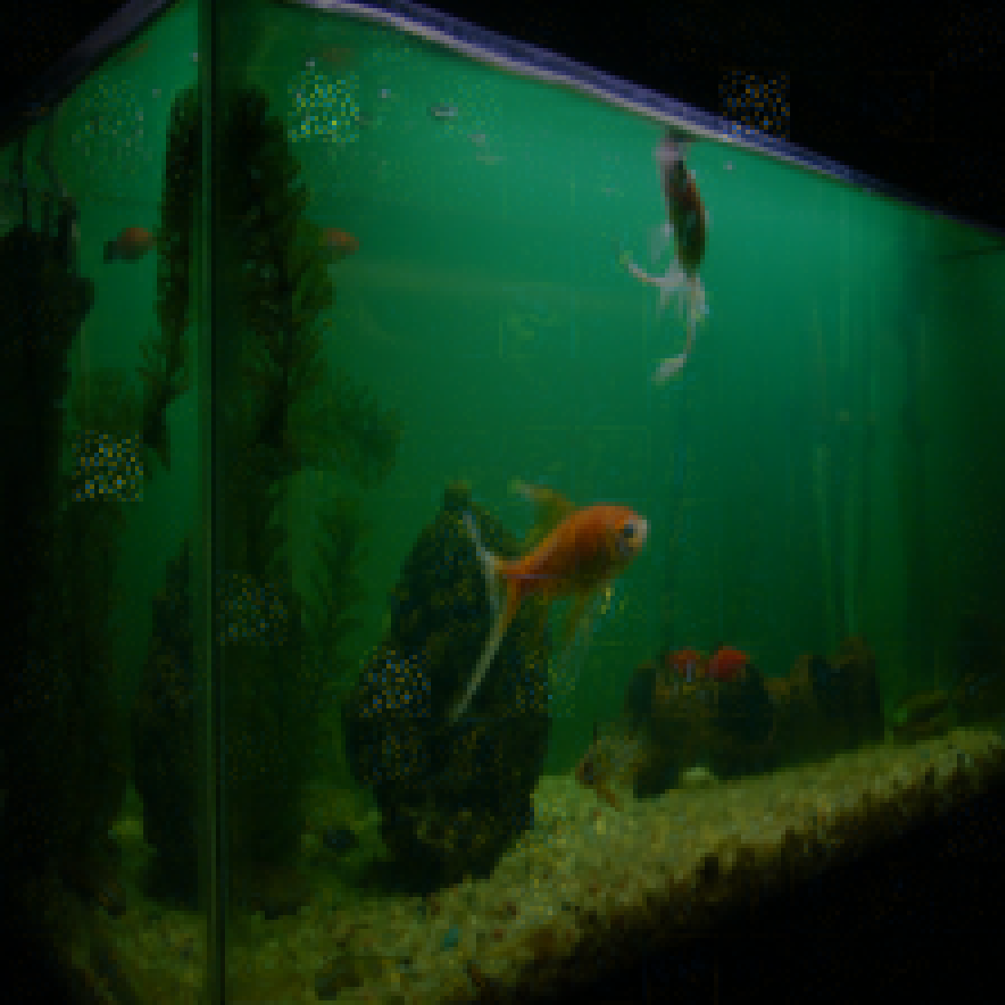

  

  FRESH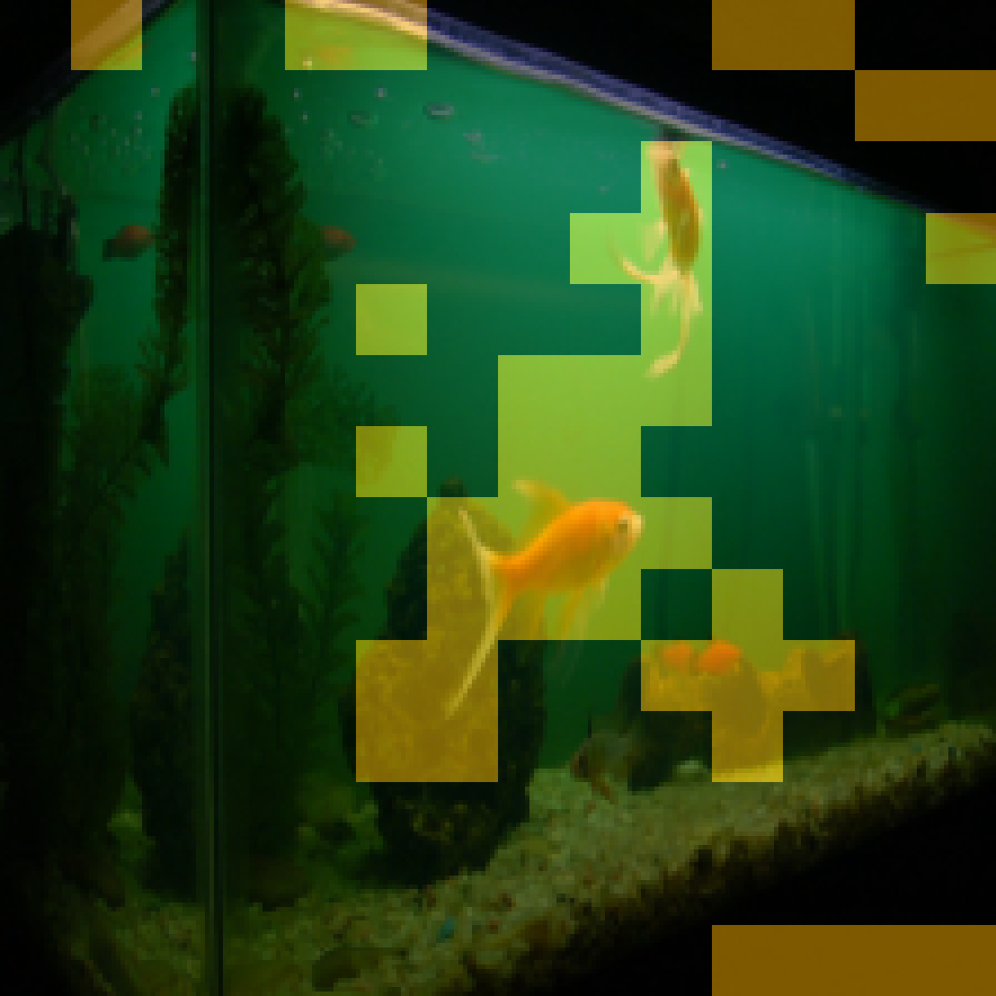

  

• LIME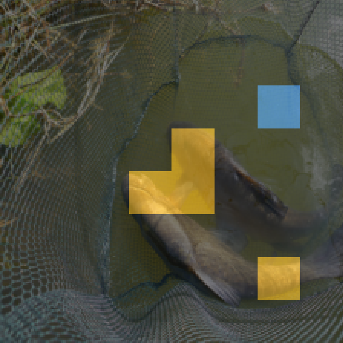

  

  SHAP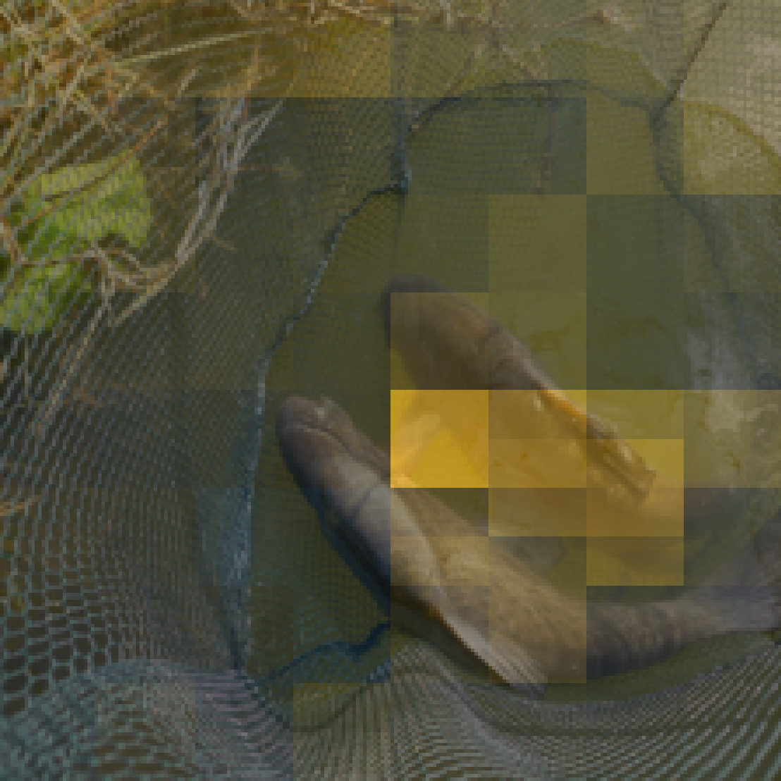

  

  RISE

  

  Grad-CAM

  

  IntGrad

  

  FRESH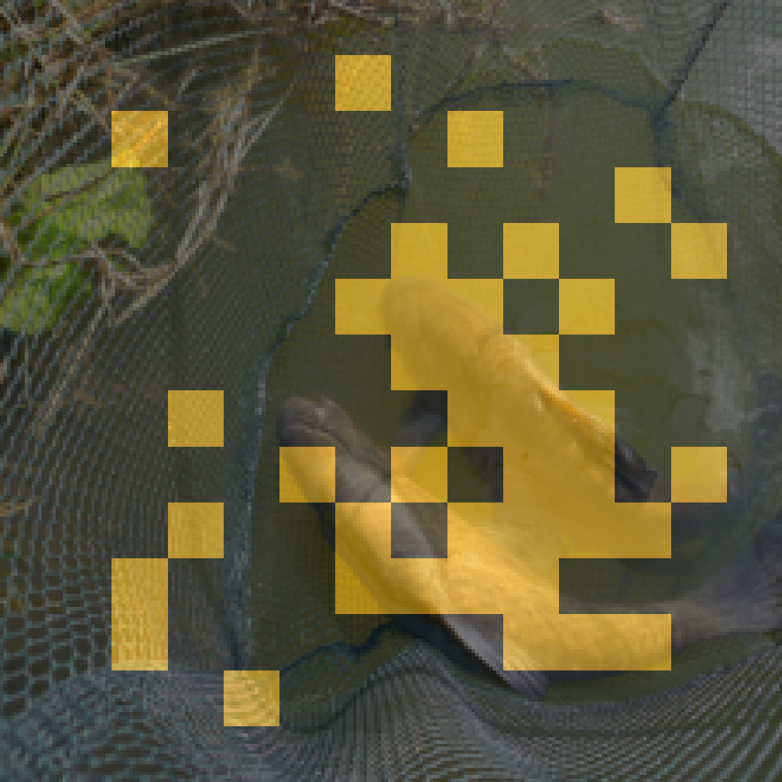

  

• LIME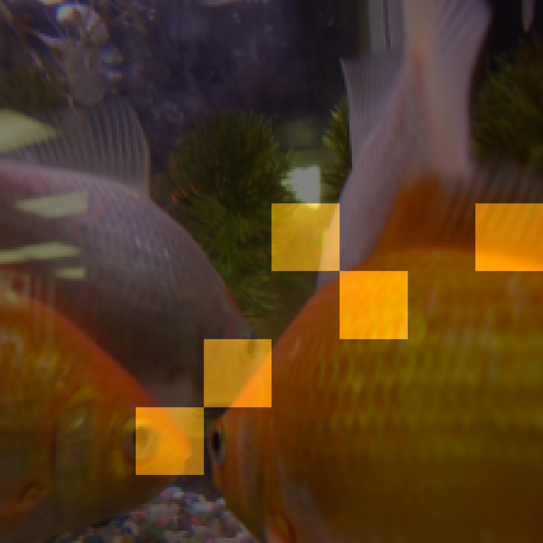

  

  SHAP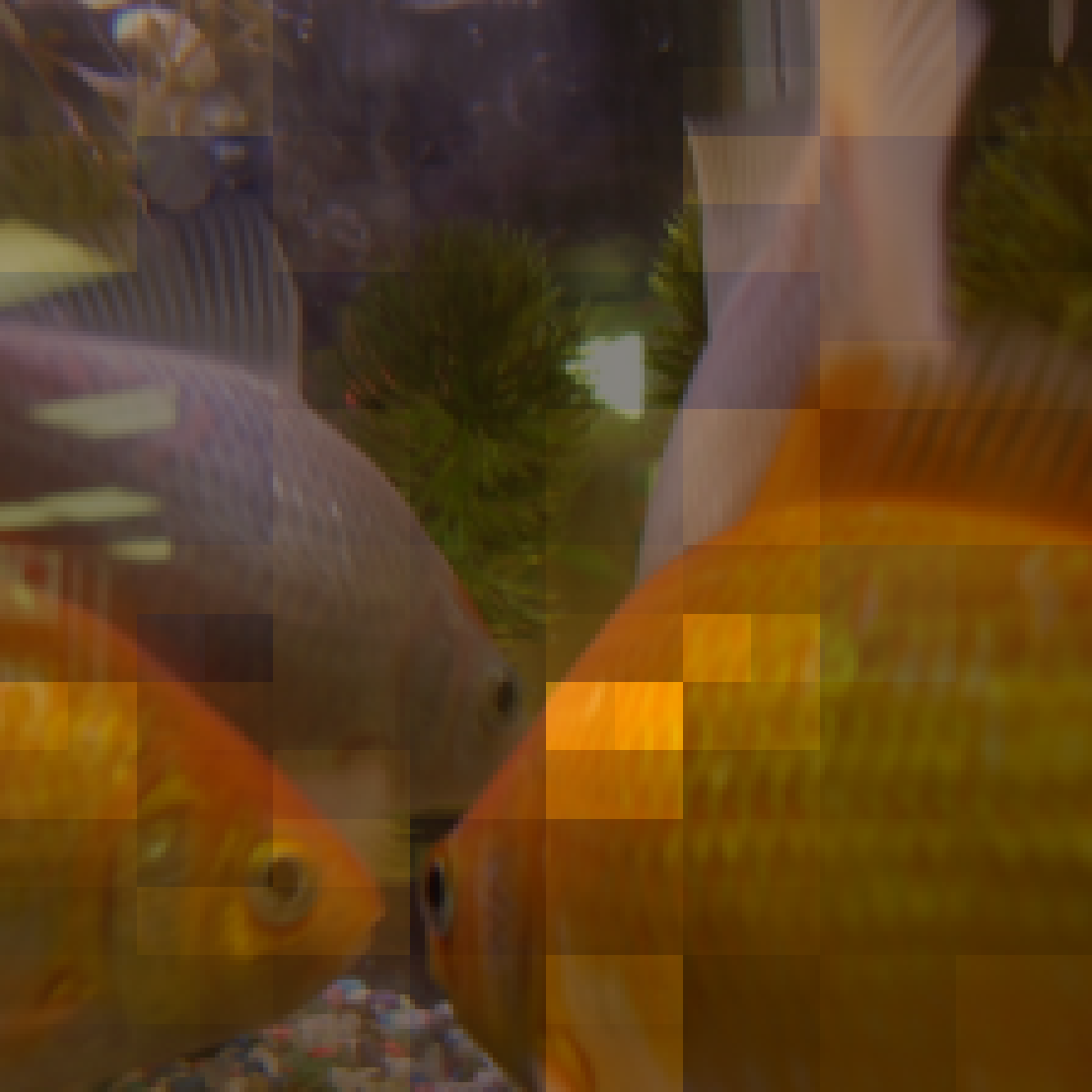

  

  RISE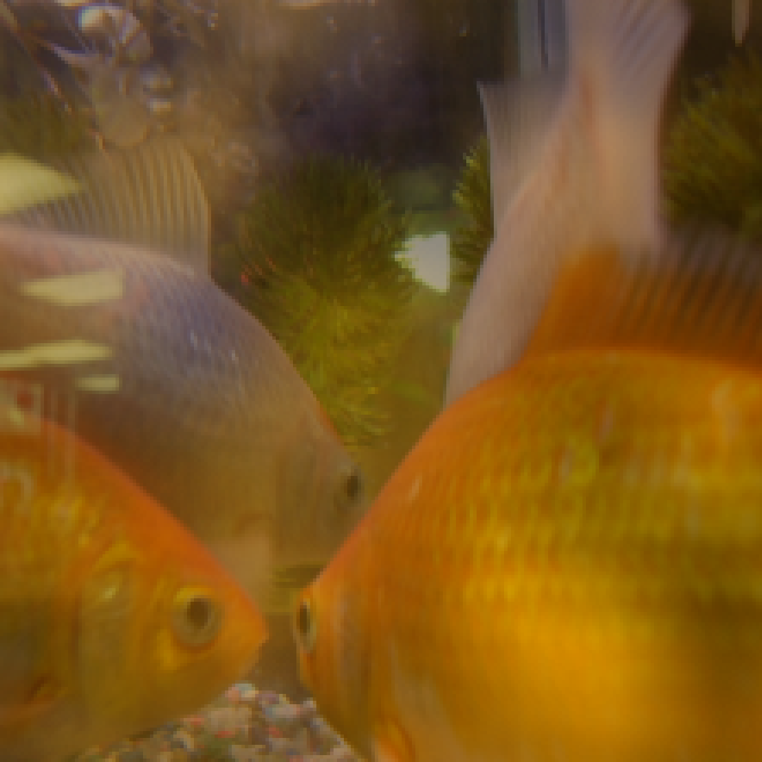

  

  Grad-CAM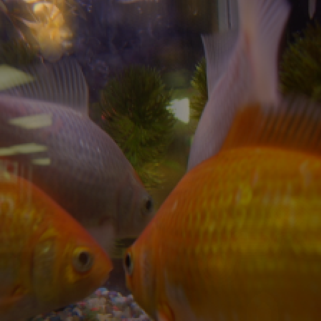

  

  IntGrad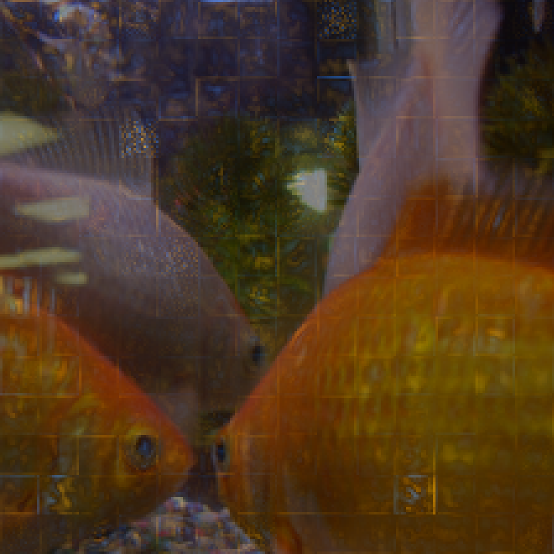

  

  FRESH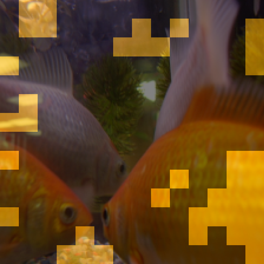

  

• LIME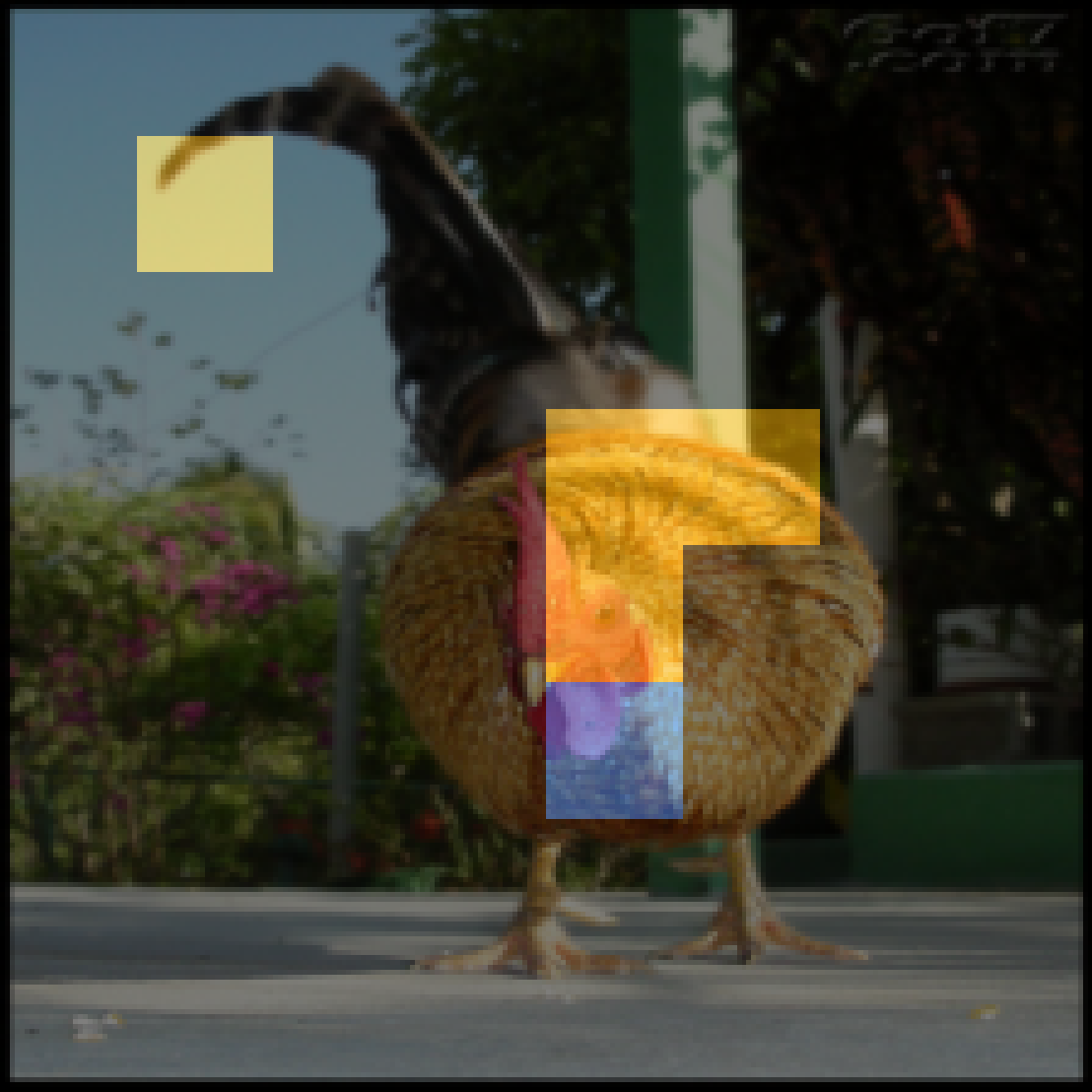

  

  SHAP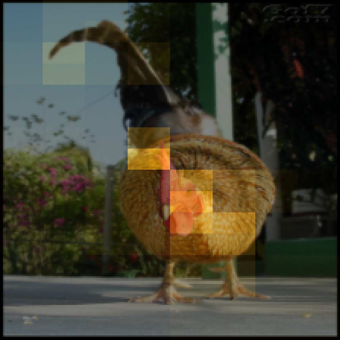

  

  RISE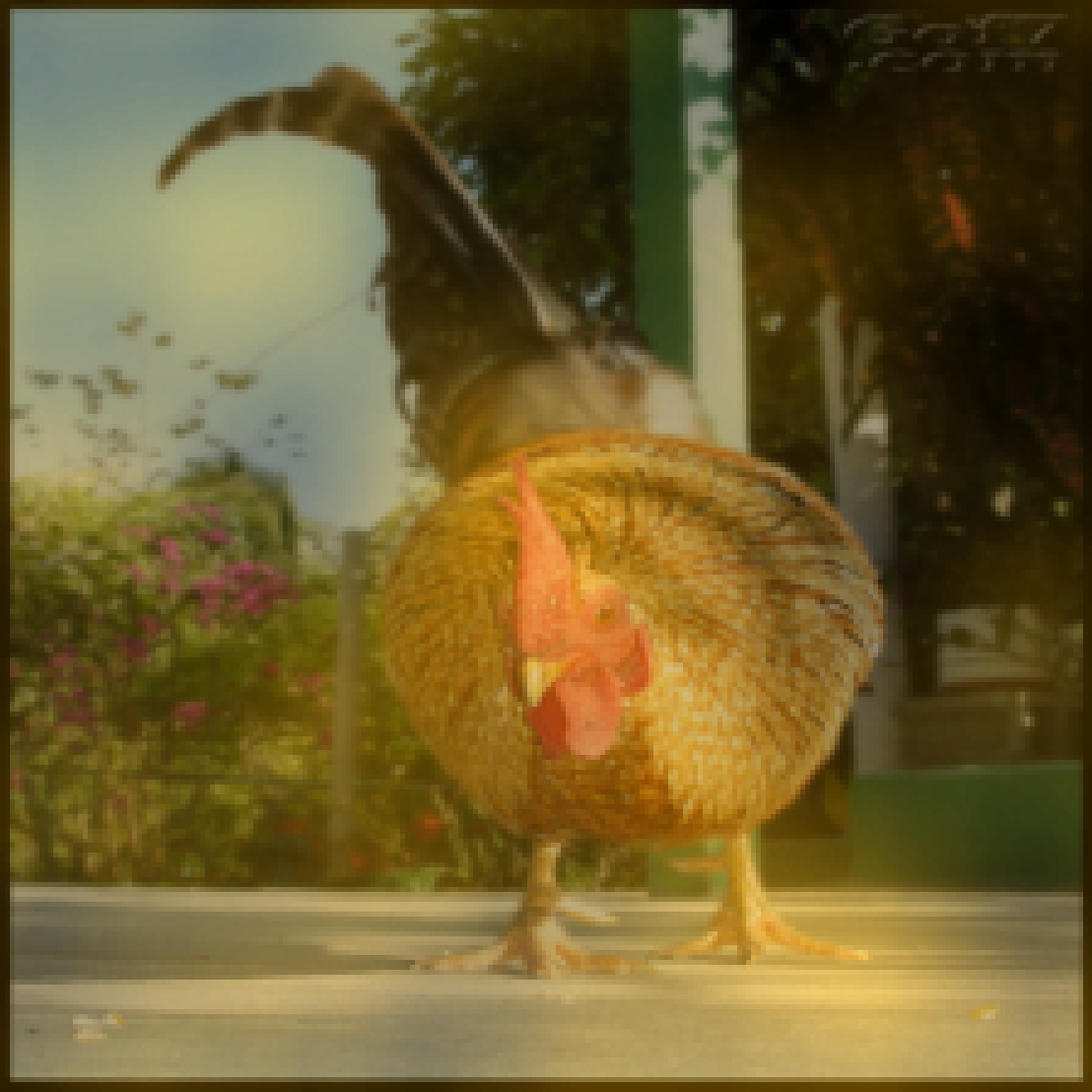

  

  Grad-CAM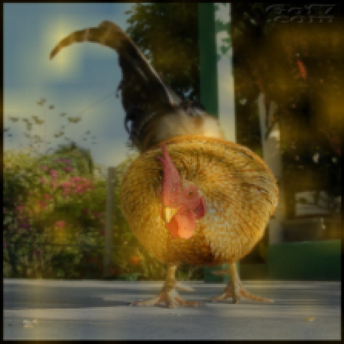

  

  IntGrad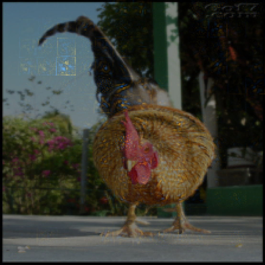

  

  FRESH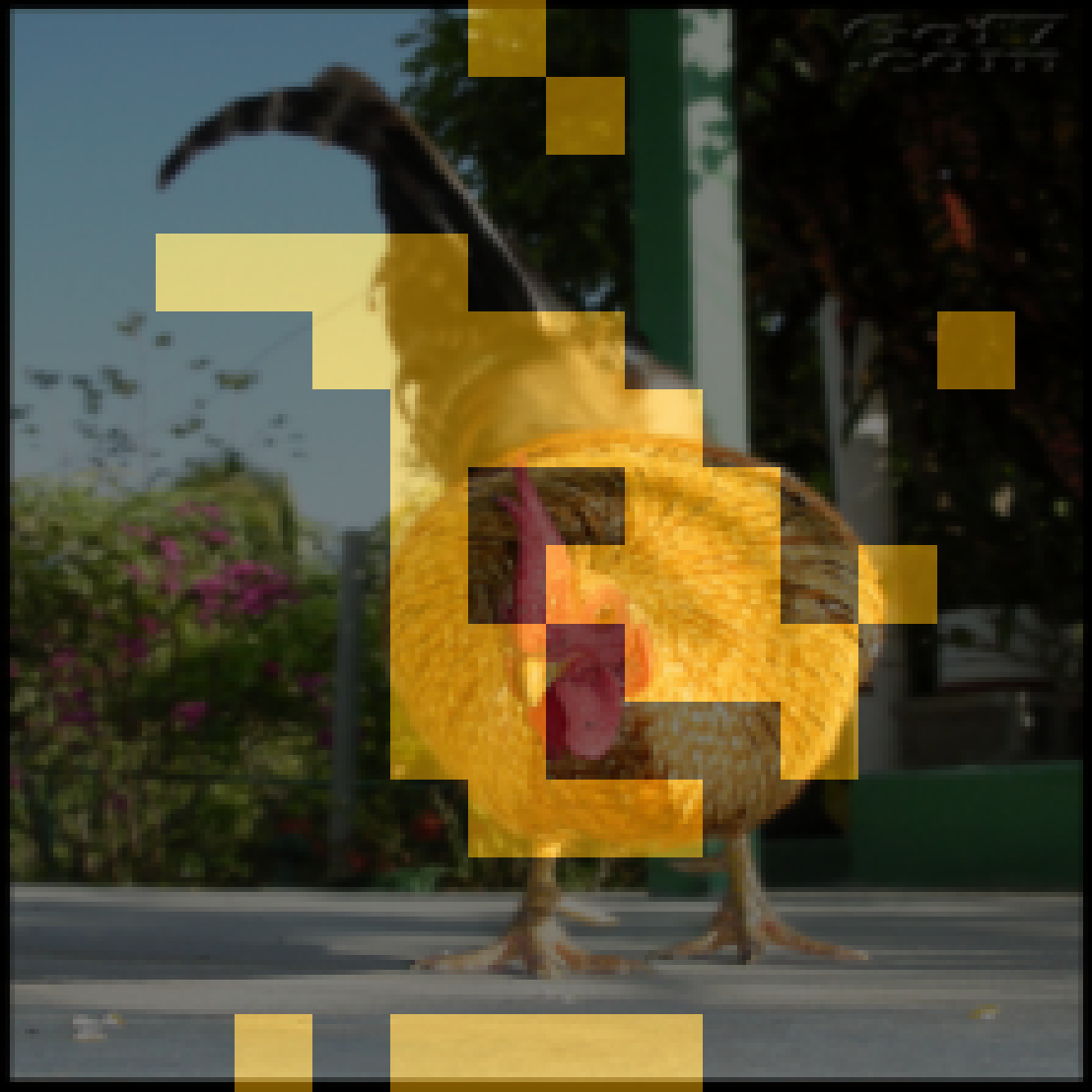

  

• LIME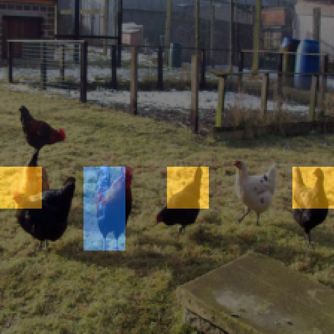

  

  SHAP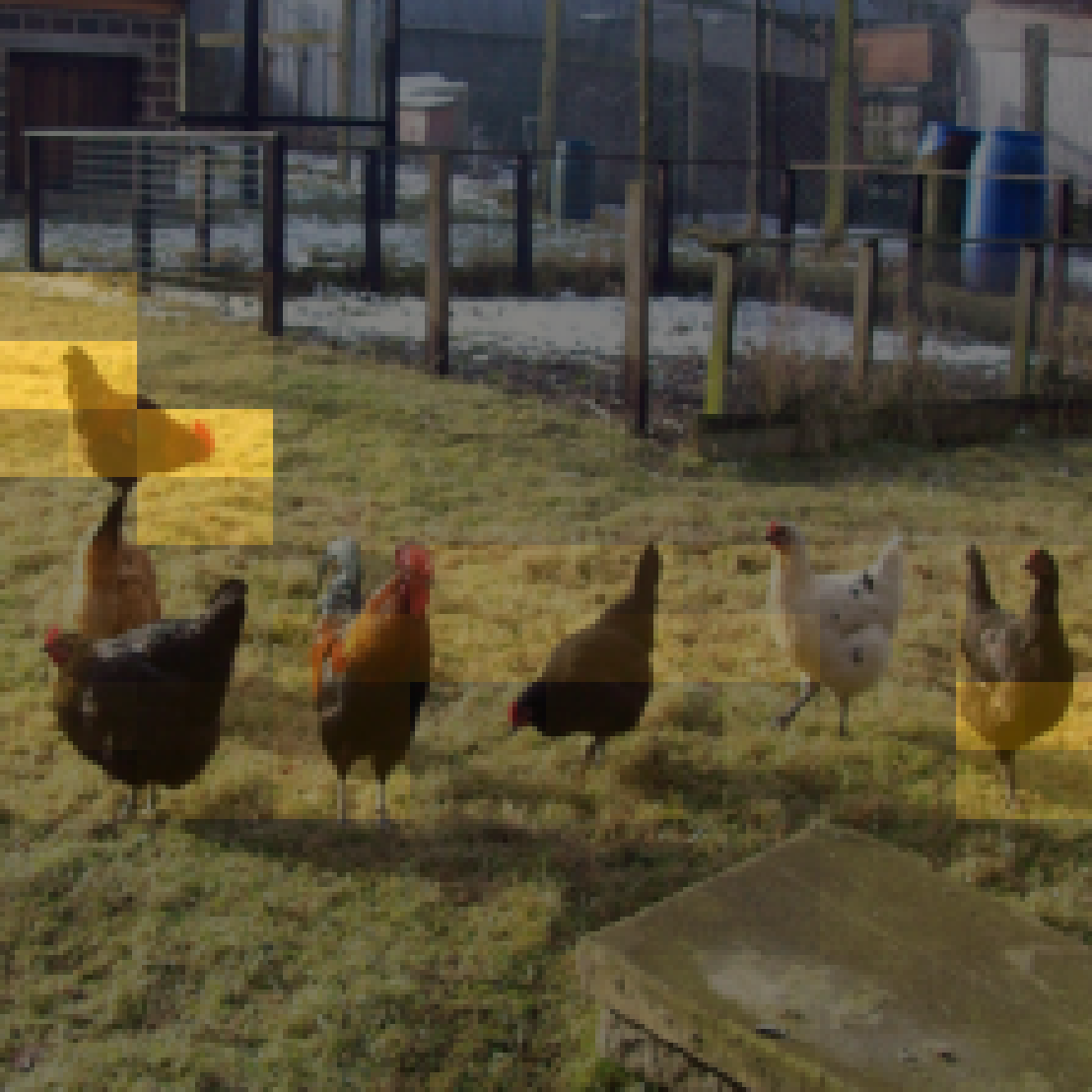

  

  RISE

  

  Grad-CAM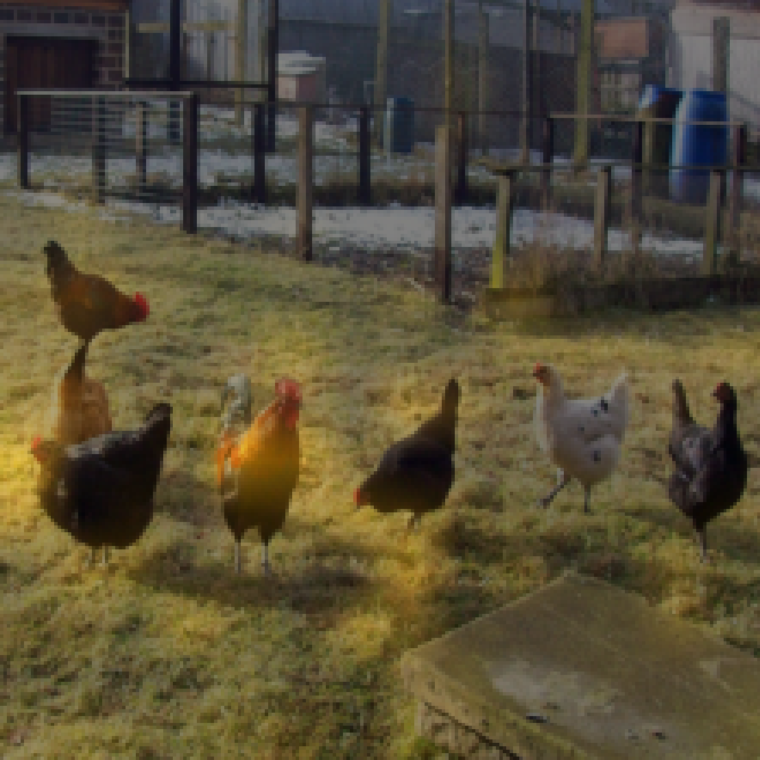

  

  IntGrad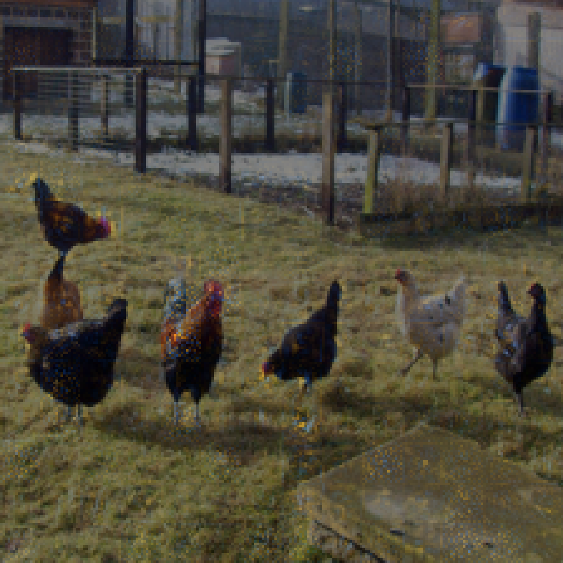

  

  FRESH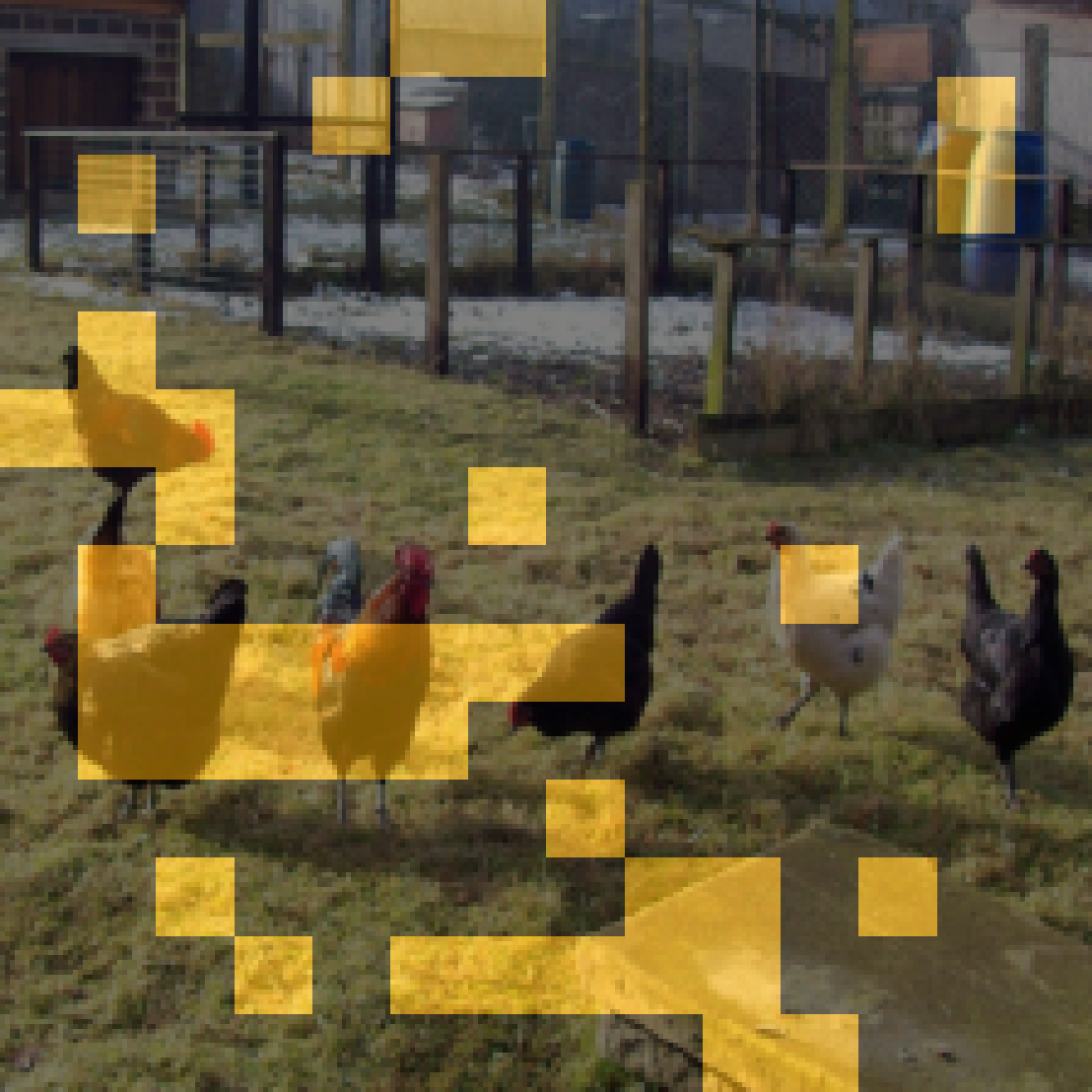

  

• LIME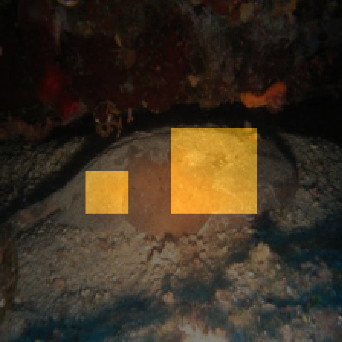

  

  SHAP

  

  RISE

  

  Grad-CAM

  

  IntGrad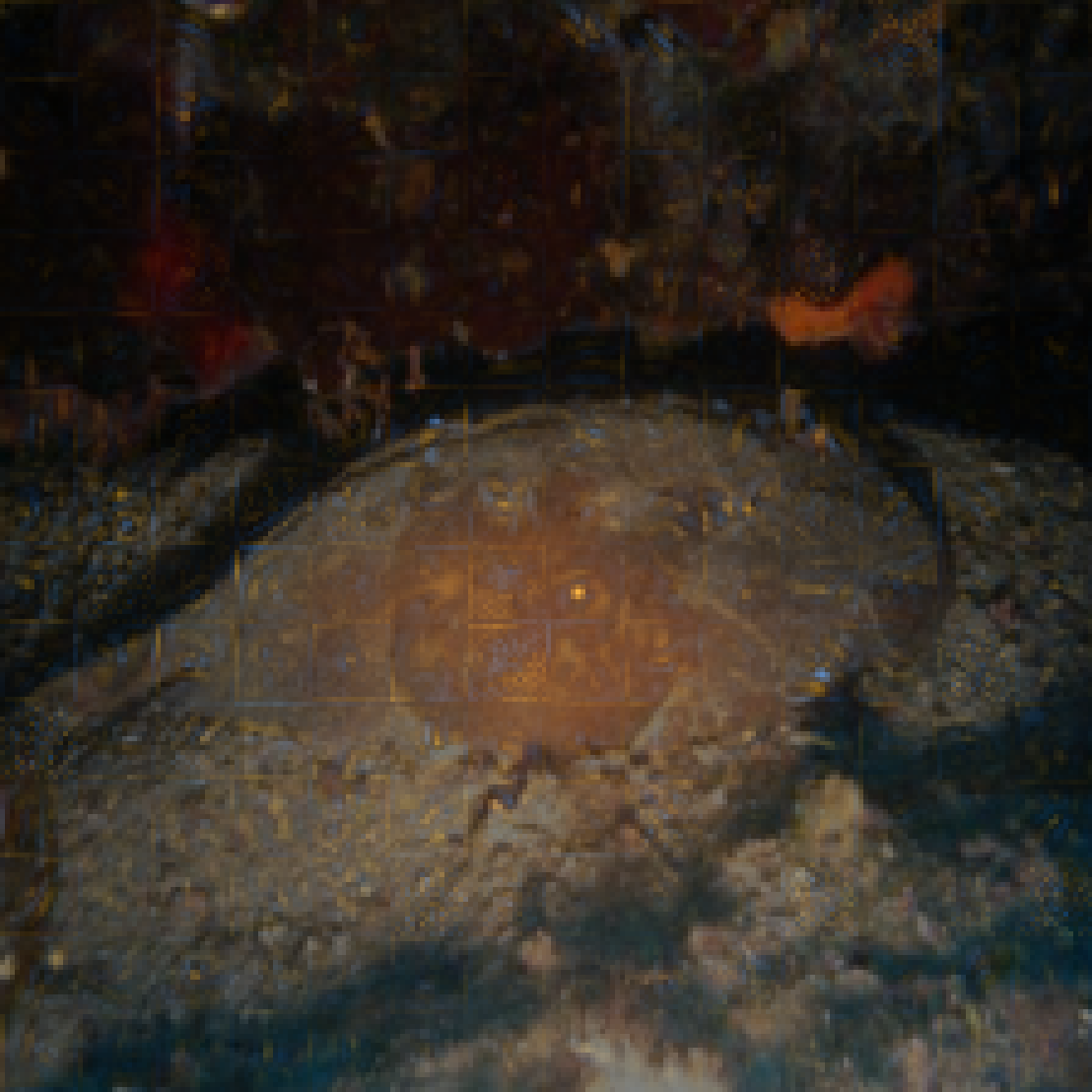

  

  FRESH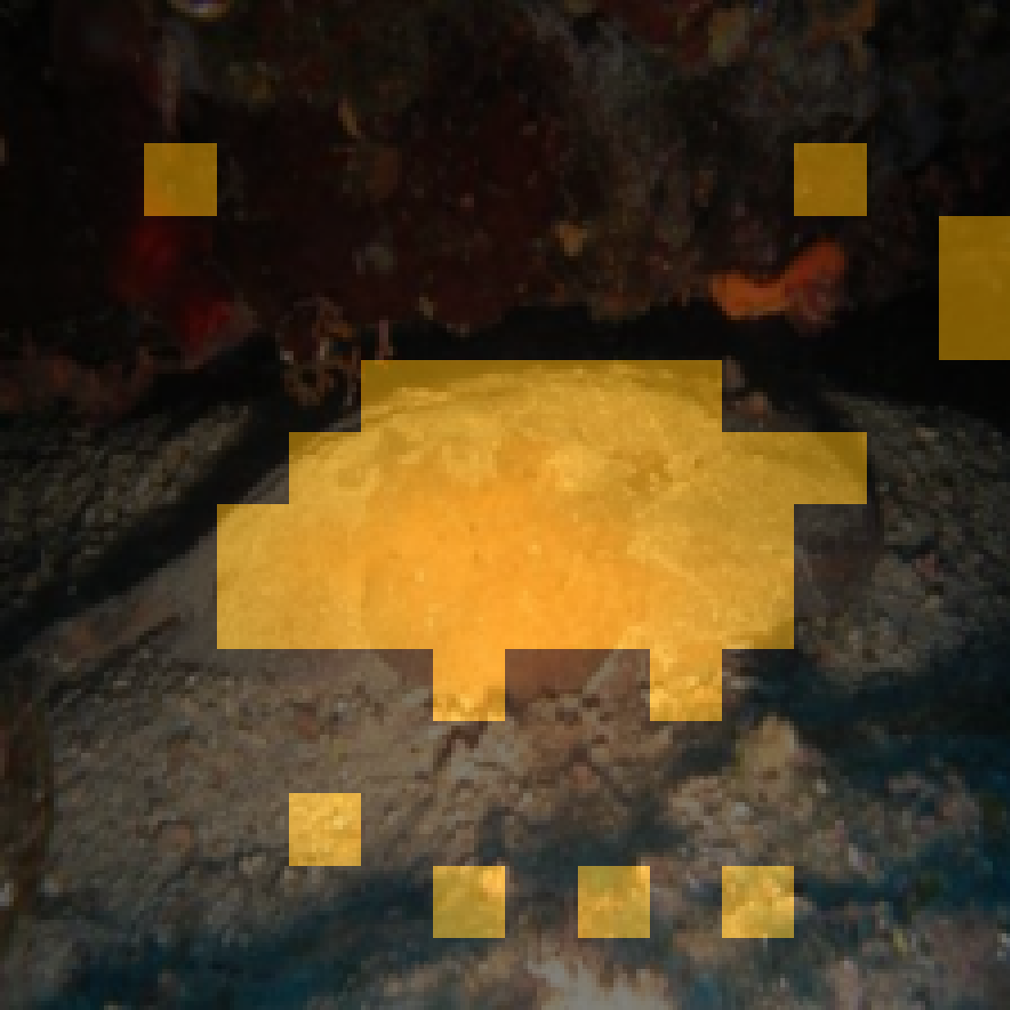

  

• LIME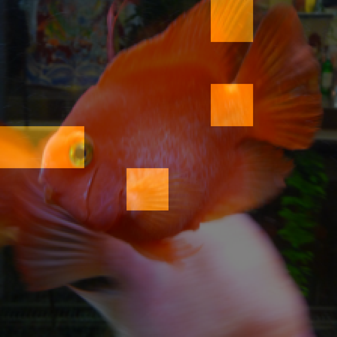

  

  SHAP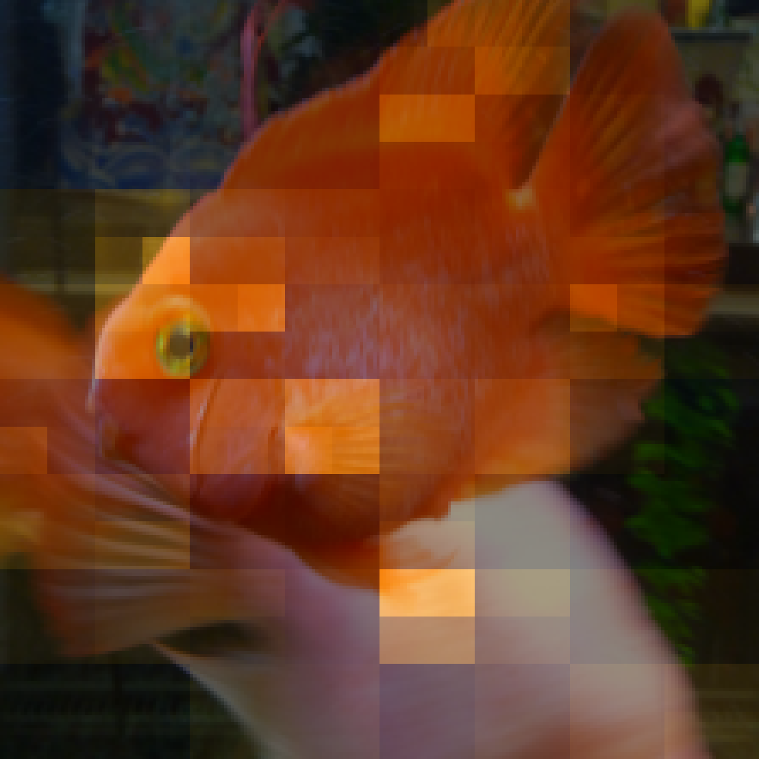

  

  RISE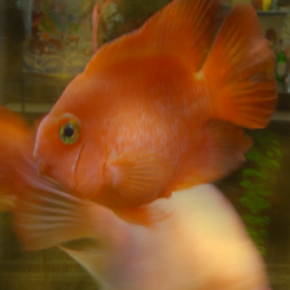

  

  Grad-CAM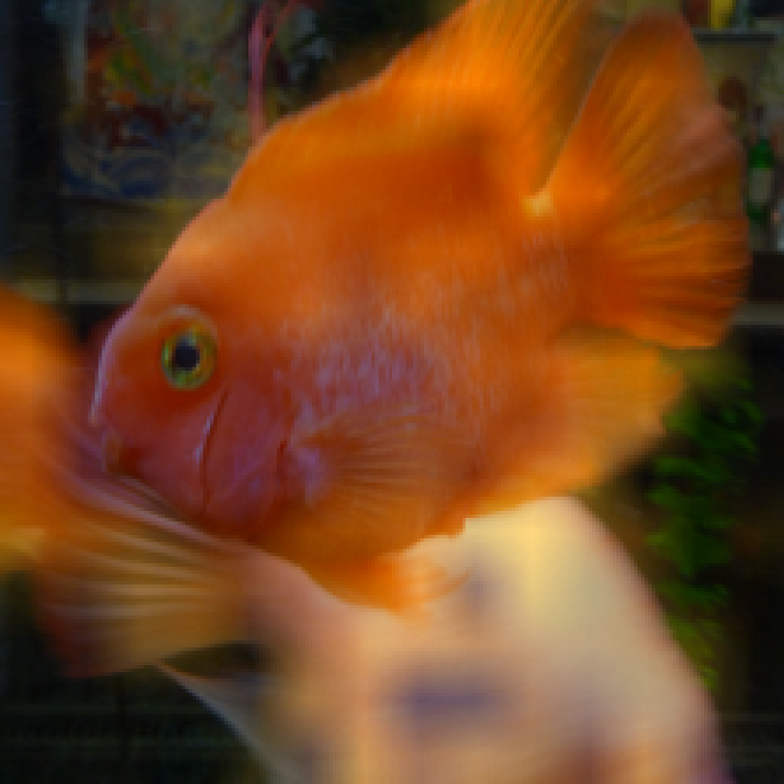

  

  IntGrad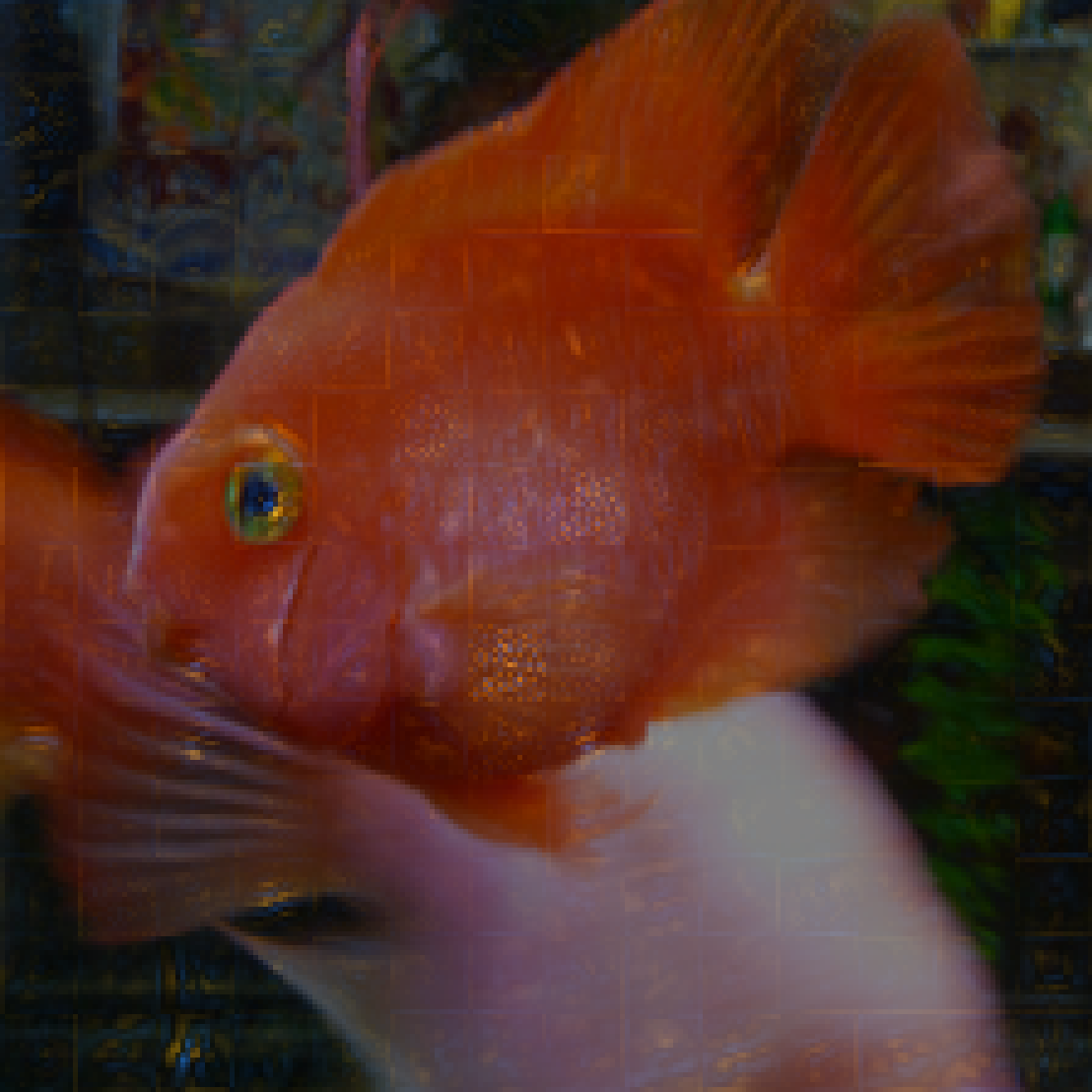

  

  FRESH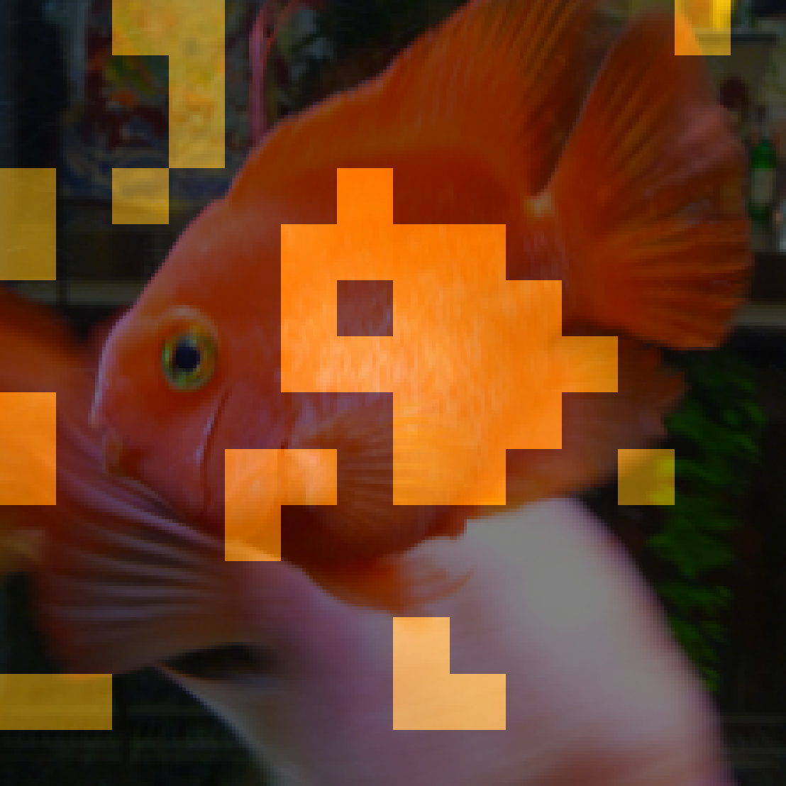

  

• LIME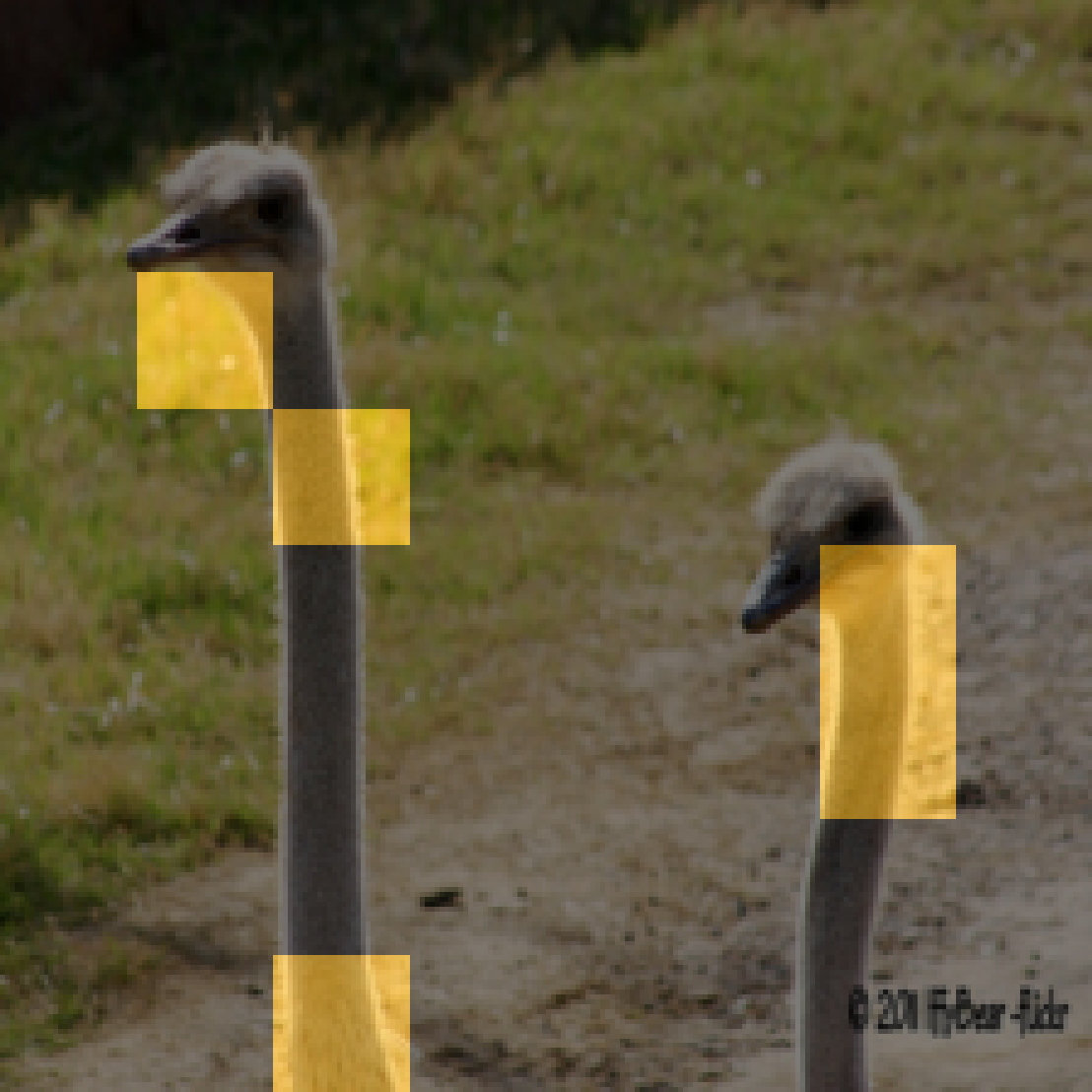

  

  SHAP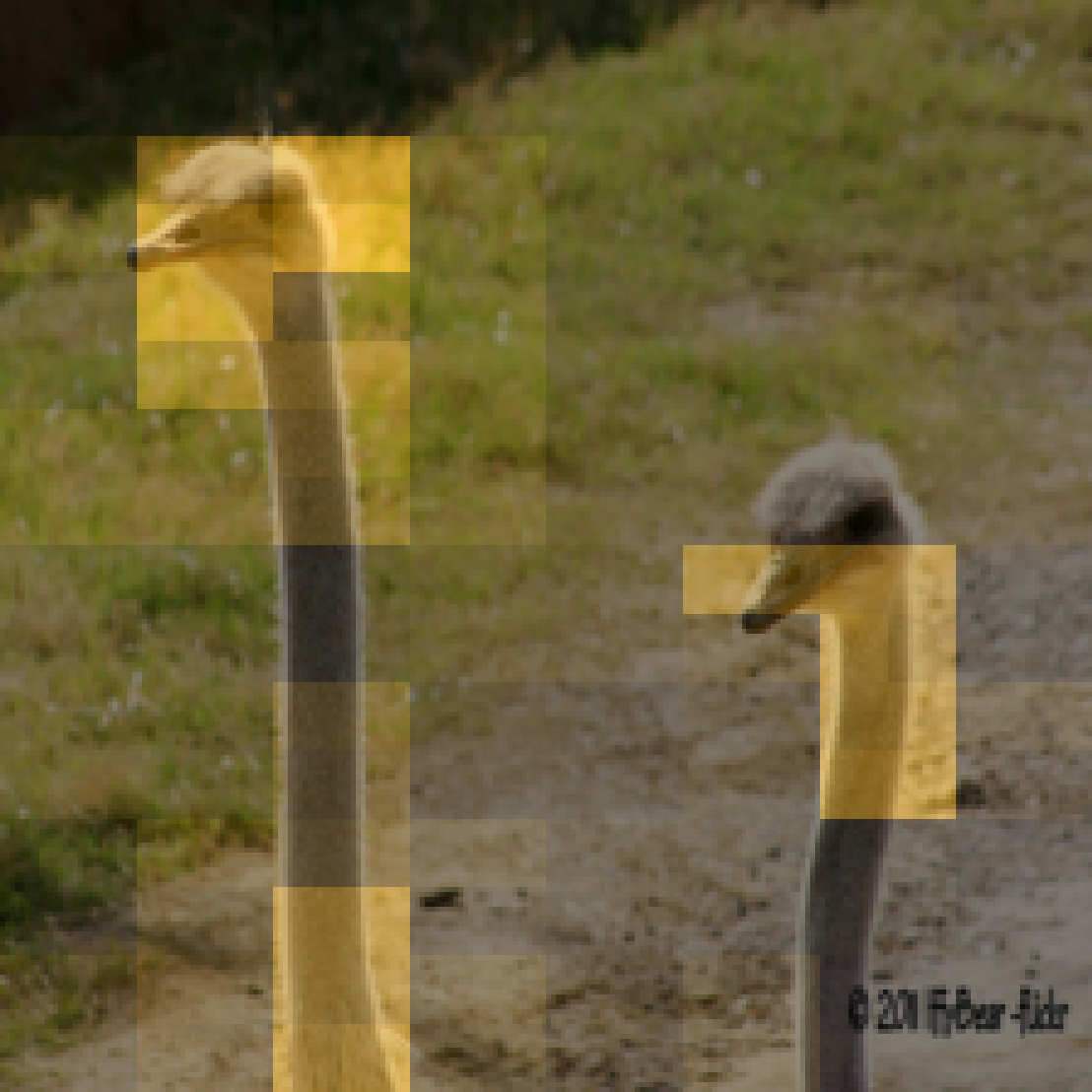

  

  RISE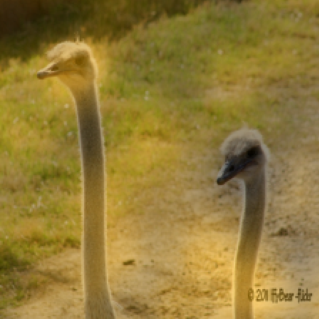

  

  Grad-CAM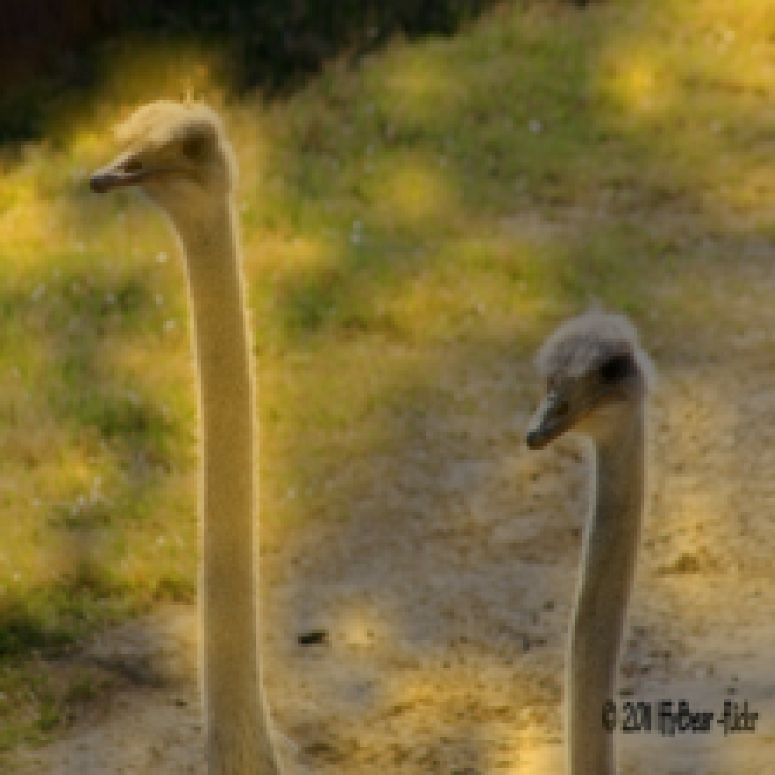

  

  IntGrad

  

  FRESH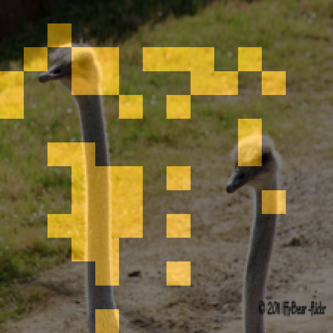

  

• LIME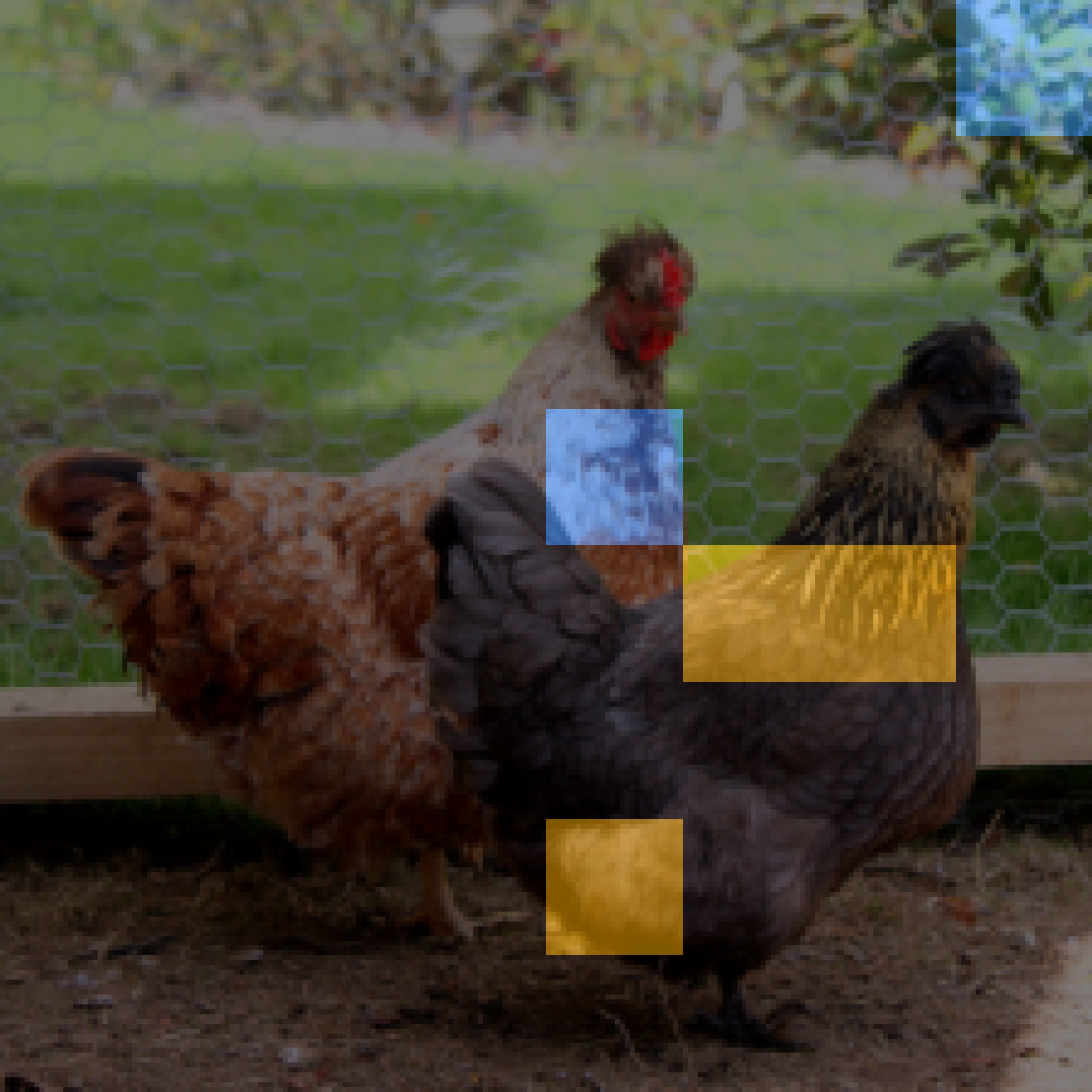

  

  SHAP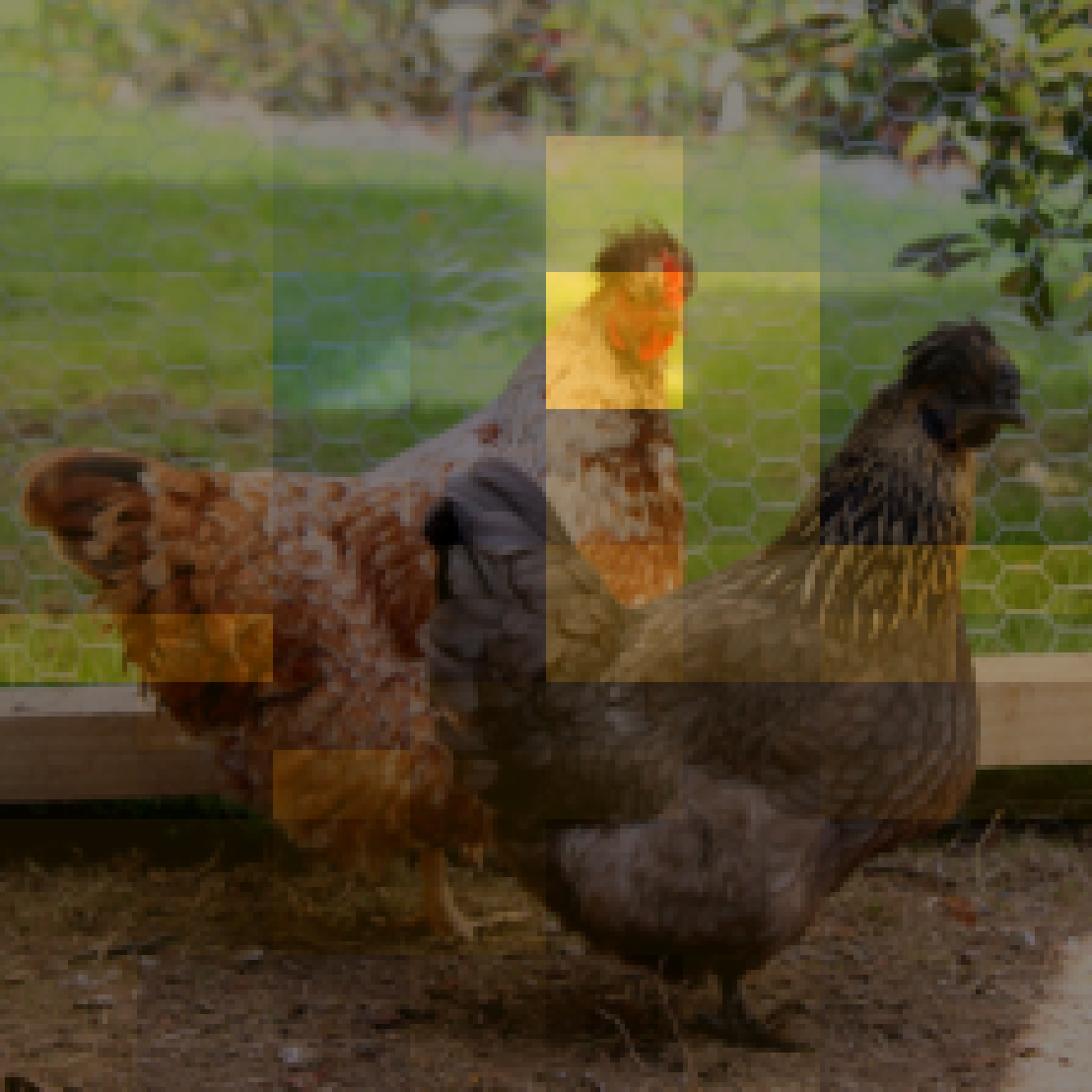

  

  RISE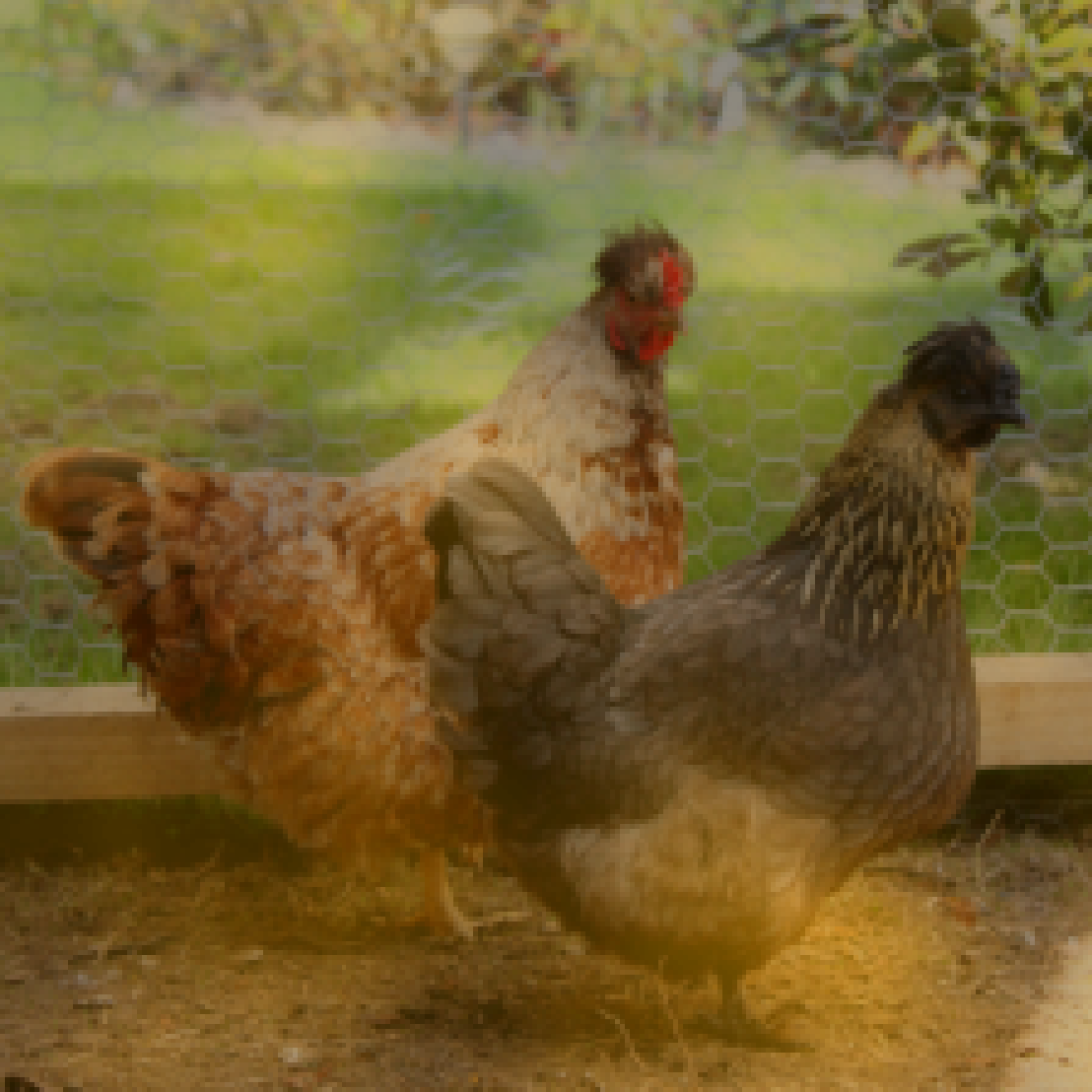

  

  Grad-CAM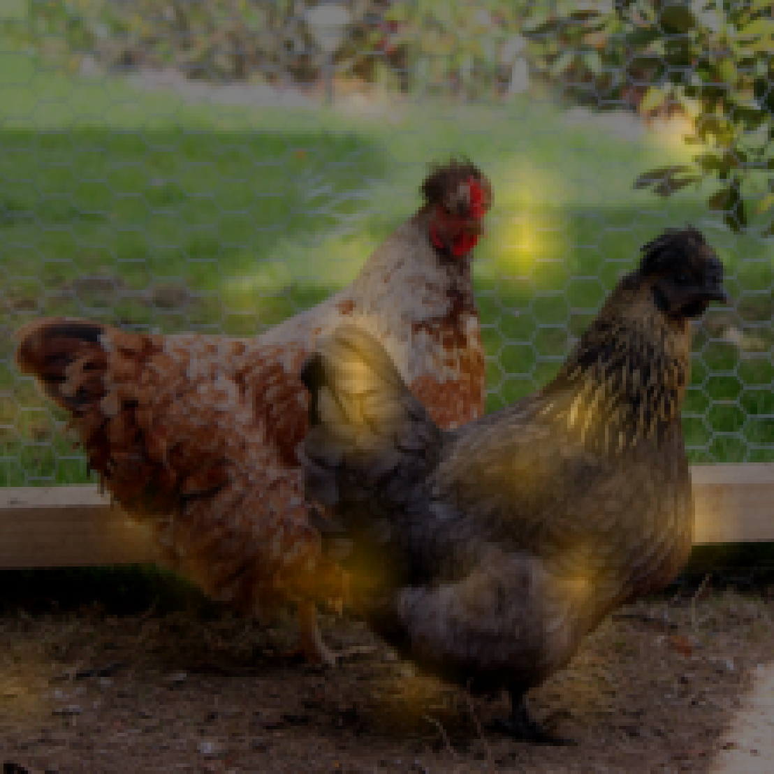

  

  IntGrad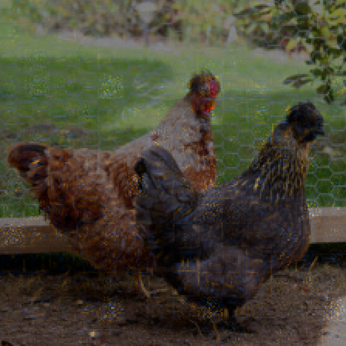

  

  FRESH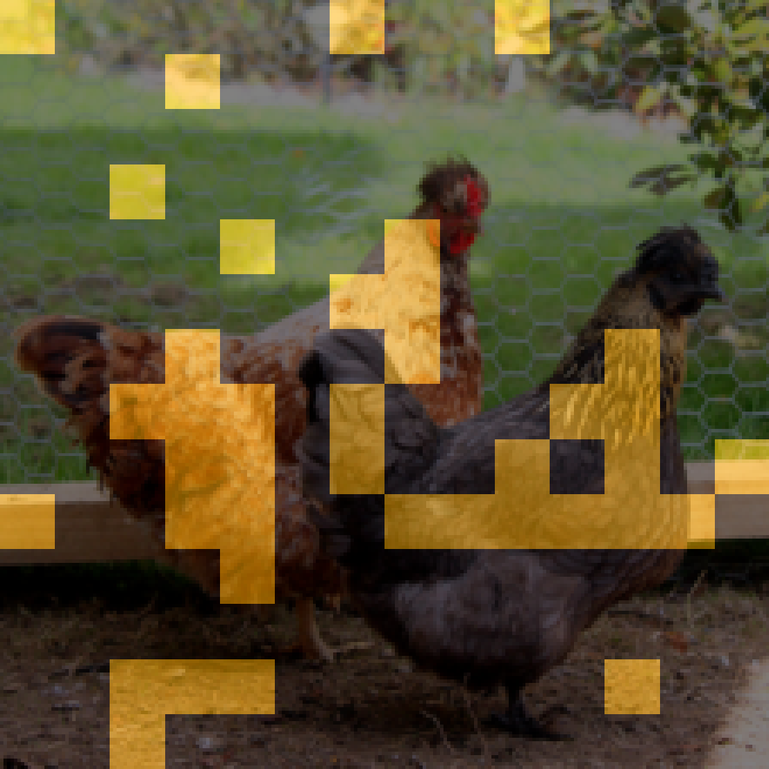

  

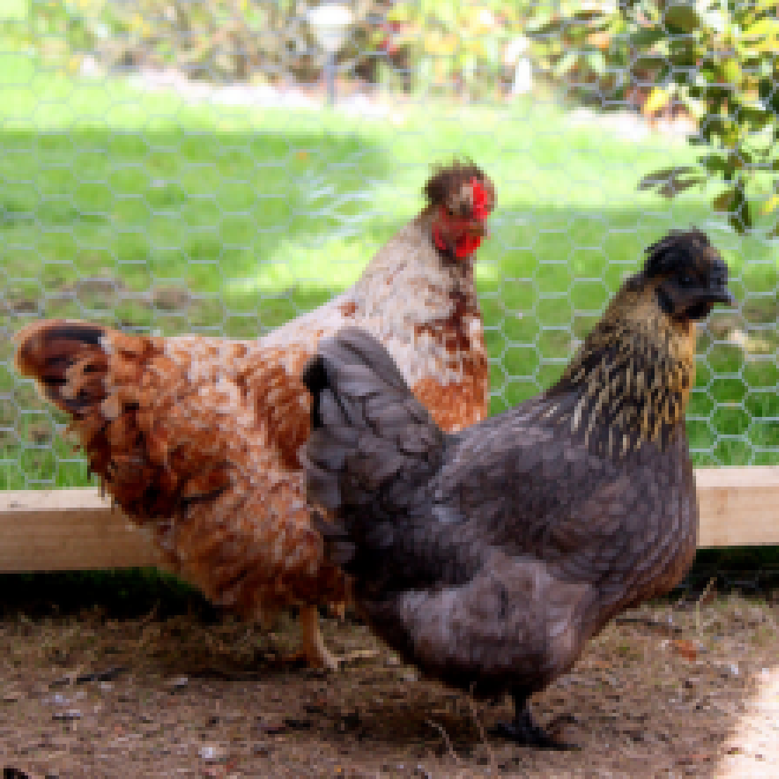
The overlaying on top of images show the feature attribution scores each attribution method. Orange overlay indicates high positive importance from the method for predicting the class, and blue overlay indicates negative importance.

The maps overlaying on top of images above show the attribution scores from different methods. LIME and SHAP build surrogate models, RISE perturb the inputs, Grad-CAM and Integrated Gradients inspect the gradients, and FRESH have the attributions built into the model. Each feature attribution method’s scores have different meanings.

Lack of Faithfulness in Feature Attributions

However, these explanations may not be “faithful”, as numerous studies have found that feature attributions fail basic sanity checks (Sundararajan et al. 2017 Adebayo et al. 2018) and interpretability tests (Kindermans et al. 2017 Bilodeau et al. 2022).

An explanation of a machine learning model is considered “faithful” if it accurately reflects the model’s decision-making process. For a feature attribution method, this means that the highlighted features should actually influence the model’s prediction.

Let’s formalize feature attributions a bit more.

Given a model $f$, an input $X$ and a prediction $y = f(X)$, a feature attribution method $\phi$ produces $\alpha = \phi(x)$. Each score $\alpha_i \in [0, 1]$ indicates the level of importance of feature $X_i$ in predicting $y$.

For example, if $\alpha_1 = 0.7$ and $\alpha_2 = 0.2$, then it means that feature $X_1$ is more important than $X_2$ for predicting $y$.

Curse of Dimensionality in Faithfulness Tests

We now discuss how feature attributions may be fundamentally unable to achieve faithfulness.

One widely-used test of faithfulness is insertion. It measures how well the total attribution from a subset of features $S$ aligns with the change in model prediction when we insert the features $X_S$ into a blank image.

For example, if a feature $X_i$ is considered to contribute $\alpha_i$ to the prediction, then adding it to a blank image should add $\alpha_i$ amount to the prediction. The total attribution scores for all features in a subset $i\in S$ is then \(\sum_{i\in S} \alpha_i\).

Definition. (Insertion error) The insertion error of an feature attribution $\alpha\in\mathbb R^d$ for a model $f:\mathbb R^d\rightarrow\mathbb R$ when inserting a subset of features $S$ from an input $X$ is

$$ \mathrm{InsErr}(\alpha, S) = \left|f(X_{S}) - f(0_d) - \sum_{i\in S} \alpha_i\right| \\ \quad\textrm{where}\;\; (X_{S})_j = \begin{cases} X_j \quad \text{if}\;\; j \in S\\ 0 \quad \text{otherwise} \end{cases} $$

The total insertion error is $\sum_{S\in\mathcal{P}} \mathrm{InsErr}(\alpha,S)$ where $\mathcal P$ is the powerset of \(\{1,\dots, d\}\).

Intuitively, a faithful attribution score of the $i$th feature should reflect the change in model prediction after the $i$th feature is added and thus have low insertion error.

Can we achieve this low insertion error though? Let’s look at this simple example of binomials:

Theorem 1 Sketch. (Insertion Error for Binomials) Let \(p:\{0,1\}^d\rightarrow \{0,1,2\}\) be a multilinear binomial polynomial function of $d$ variables. Furthermore suppose that the features can be partitioned into $(S_1,S_2,S_3)$ of equal sizes where $p(X) = \prod_{i\in S_1 \cup S_2} X_i + \prod_{j\in S_2\cup S_3} X_j$. Then, there exists an $X$ such that any feature attribution for $p$ at $X$ will incur exponential total insertion error.

When features are highly correlated such as in a binomial, attributing to individual features separately fails to give low insertion error, and thus fails to faithfully represent features’ contributions to the prediction.

Grouped Attributions Overcome Curse of Dimensionality

Highly correlated features cannot be individually faithful. Our approach is then to group these highly correlated features together.

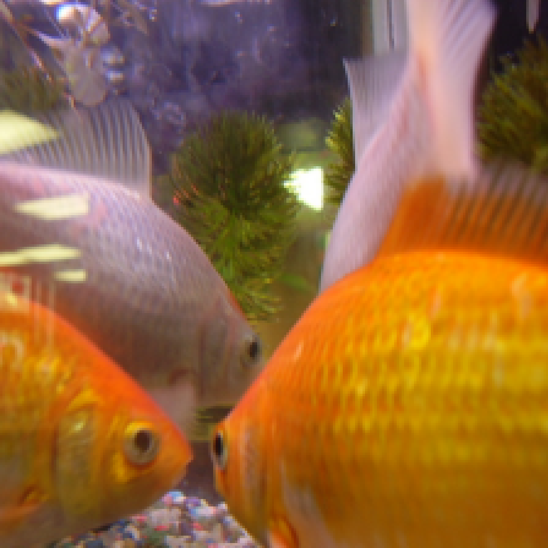
We investigate grouped attributions as a different type of attributions, which assign scores to groups of features instead of individual features. A group only contributes its score if all of its features are present, as shown in the following example for images.

Visualization of grouped attributions. For a set of group attributions, scores are assigned to groups of features instead of individual features. The score for each group represents how much each group of features together contributes to the prediction of a class. We can see that masks can be interpreted as objects kept and objects removed. In this example, group 2, which includes the fish and the predator, contributes 15% to predicting “tench”, while group \(G\), which has the fish and dark lines removed, contributes only 1% to predicting “tench”, but 21% to predicting “Rooster”.

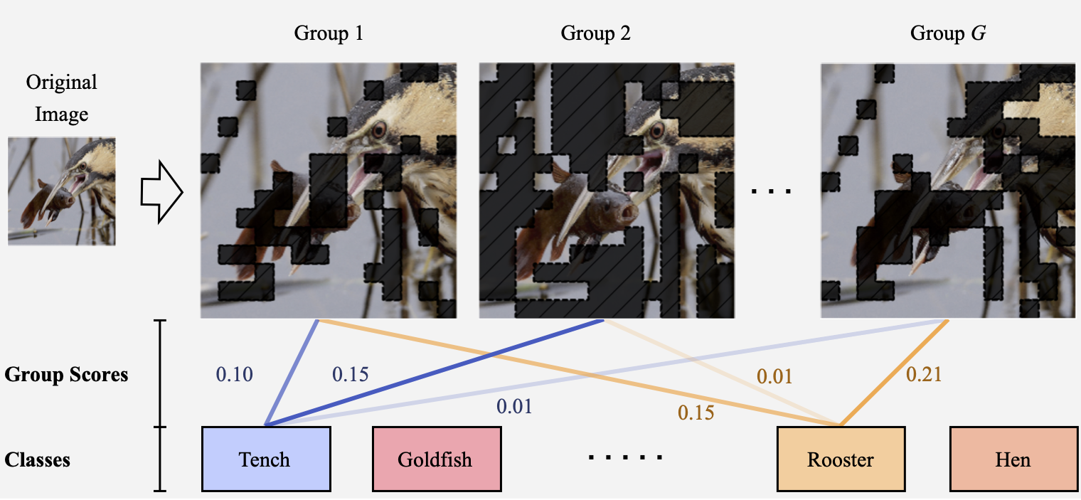
The prediction for each class \(y = f(X)\) is decomposed into $G$ scores and corresponding predictions $(c_1, y_1), \dots, (c_G, y_G)$ from groups groups $(S_1,\dots, S_G) \in [0,1]^d $. For example, scores from all the blue lines sum up to 1.0 for the class “tench” in the example above.

The concept of groups is then formalized as following:

Grouped Attribution: Let $x\in\mathbb R^d$ be an example, and let \(S_1, \dots, S_G \in \{0,1\}^d\) designate $G$ groups of features where $j \in S_i$ if feature $j$ is included in the $i$th group. Then, a grouped feature attribution is a collection $\beta = {(S_i,c_i)}_{i=1}^G$ where $c_i\in\mathbb R$ is the attributed score for the $i$th group of features $m_i$.

We can prove that there is a constant sized grouped attribution that achieves zero insertion error, when we add whole groups together using their grouped attribution scores.

Corollary. Consider the binomial from the Theorem 1 Sketch. Then, there exists a grouped attribution with zero insertion error for the binomial.

Grouped attributions can then faithfully represent contributions from groups of features. We can then overcome exponentially growing insertion errors when the features interact with each other.

Our Approach: Sum-of-Parts Models

Now that we understand the need for grouped attributions, how do we ensure they are faithful?

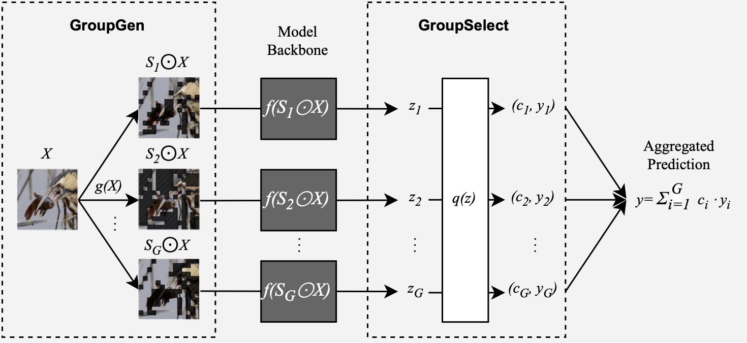
We develop Sum-of-Parts (SOP), a faithful-by-construction model that first assigns features to groups with $\mathsf{GroupGen}$ module, and then select and aggregates predictions from the groups with $\mathsf{GroupSelect}$ module.

In this way, the prediction from each group only depends on the group, and the score for a group is thus faithful to the group’s contribution.

Structure of a Sum-of-Parts model. A group generator $g$ first generates groups of features. Each group of features \(S_i\odot X\) then goes through the backbone model to obtain the group embedding \(z_i\). A group selector $q$ then assigns a score $c_i$ to each group $i$’s representation. The logits from groups are then aggregated for final prediction $y$.

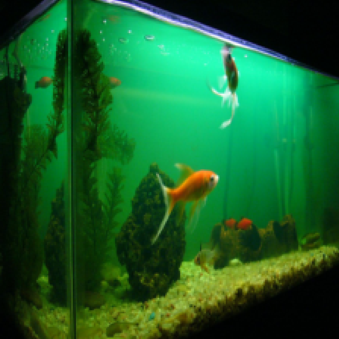
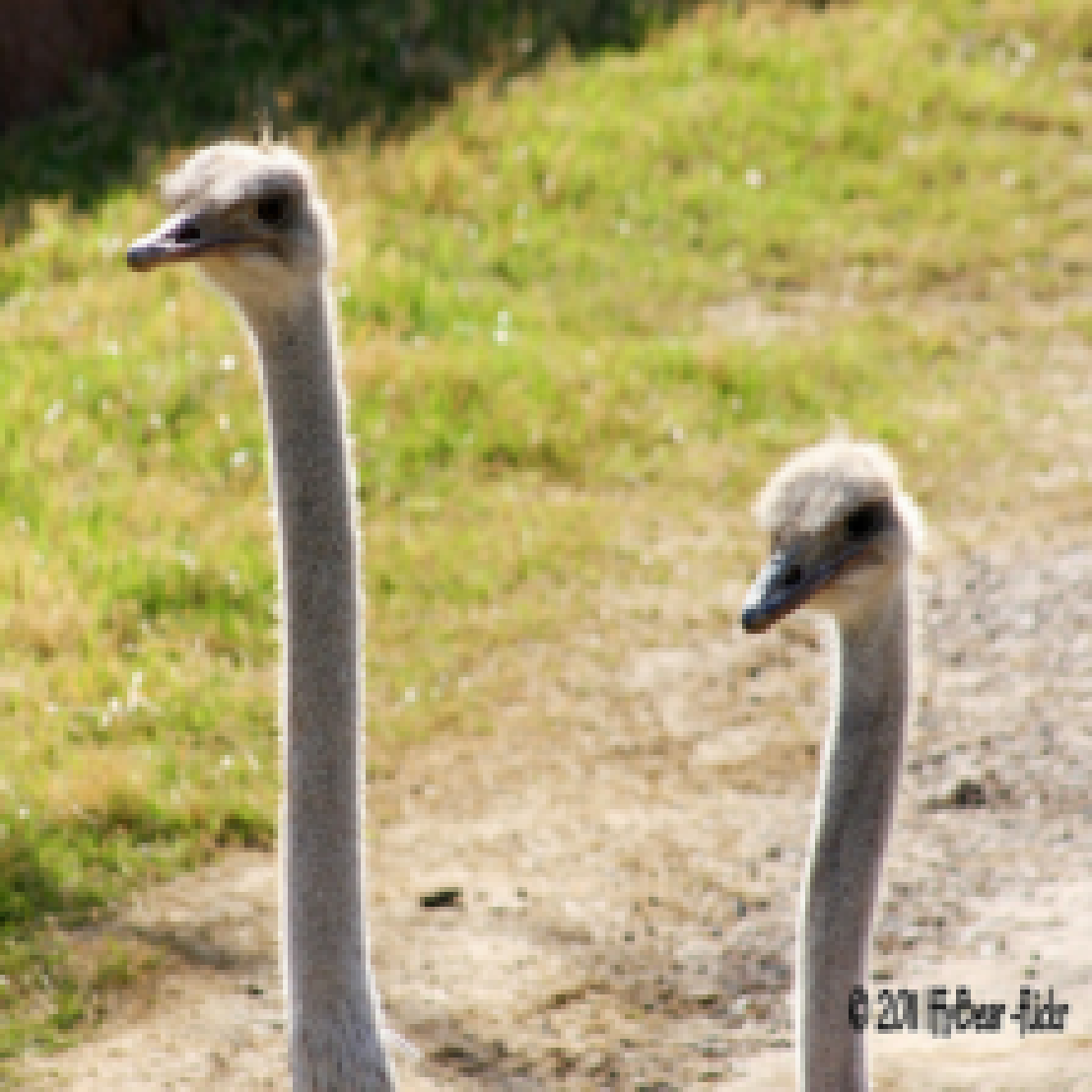
Click on thumbnails to see different example groups our model obtained for ImageNet:

• 
• 
• 
• 
• 
• 
• 
• 
• 
• 

• 0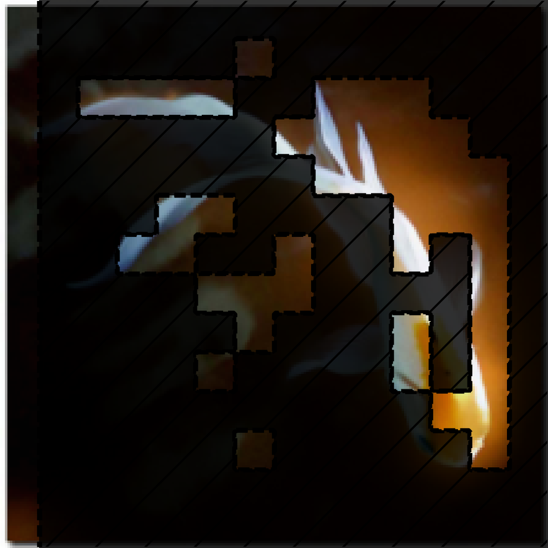

  

  1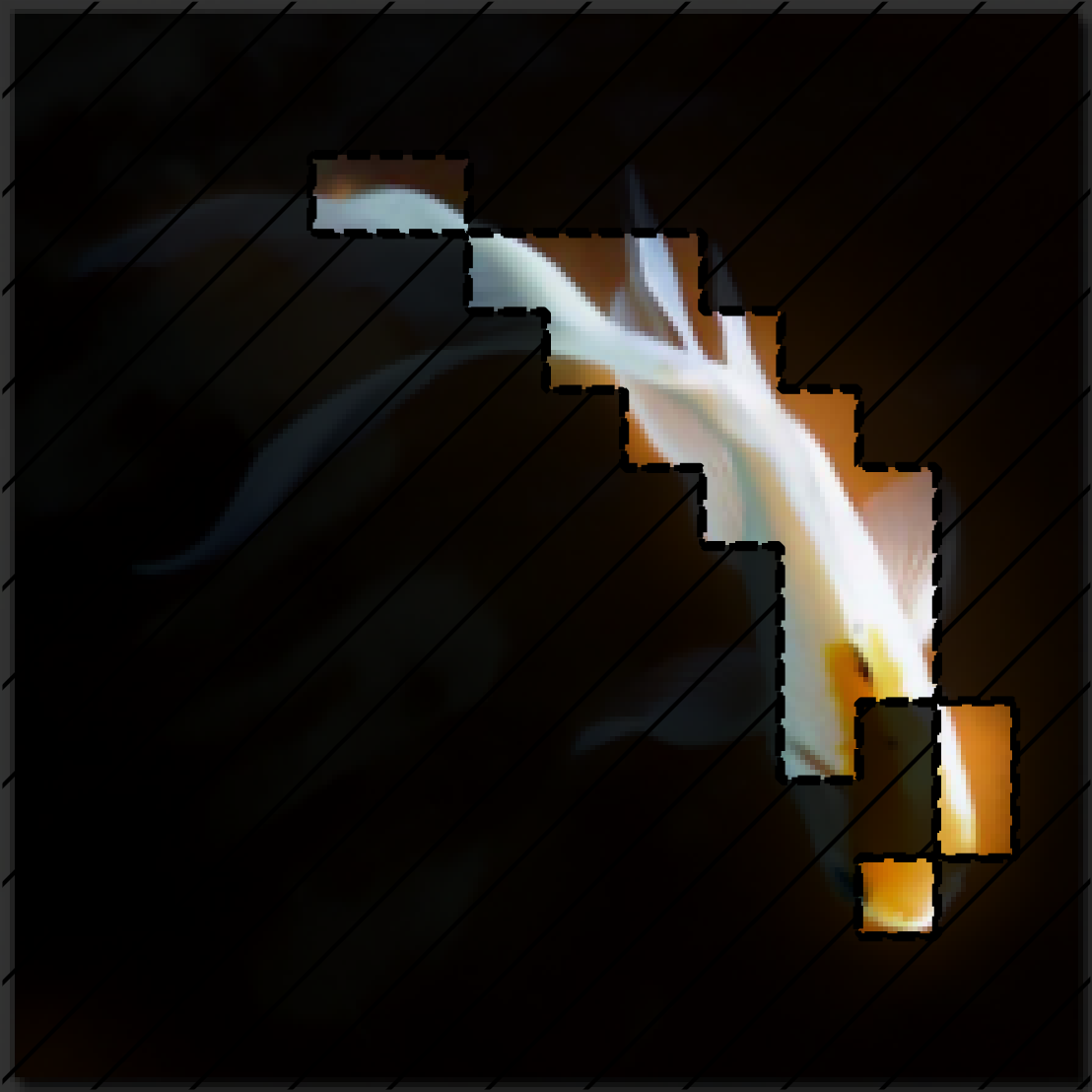

  

  2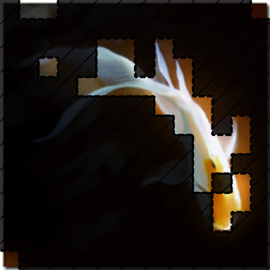

  

  0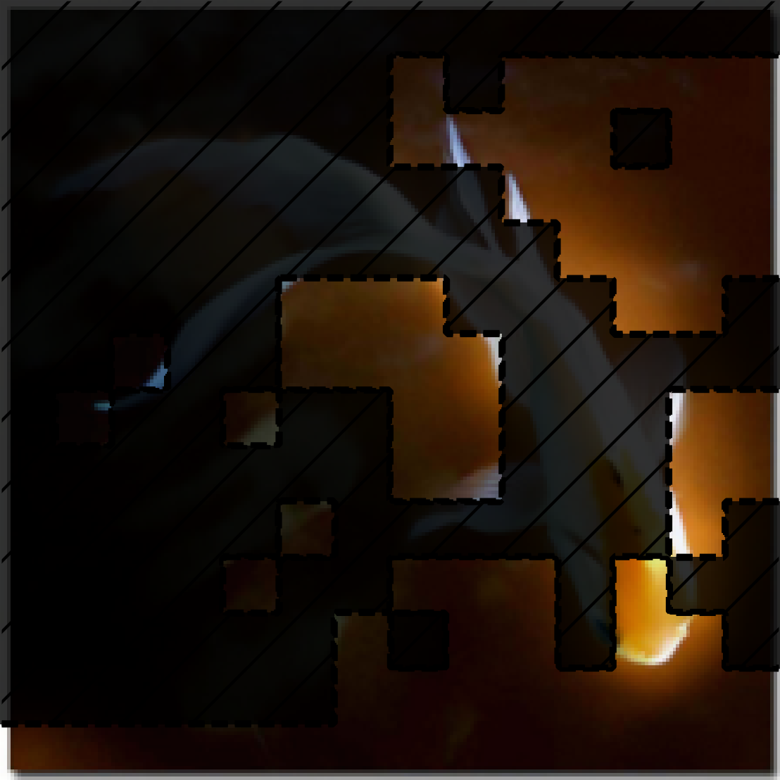

  

  1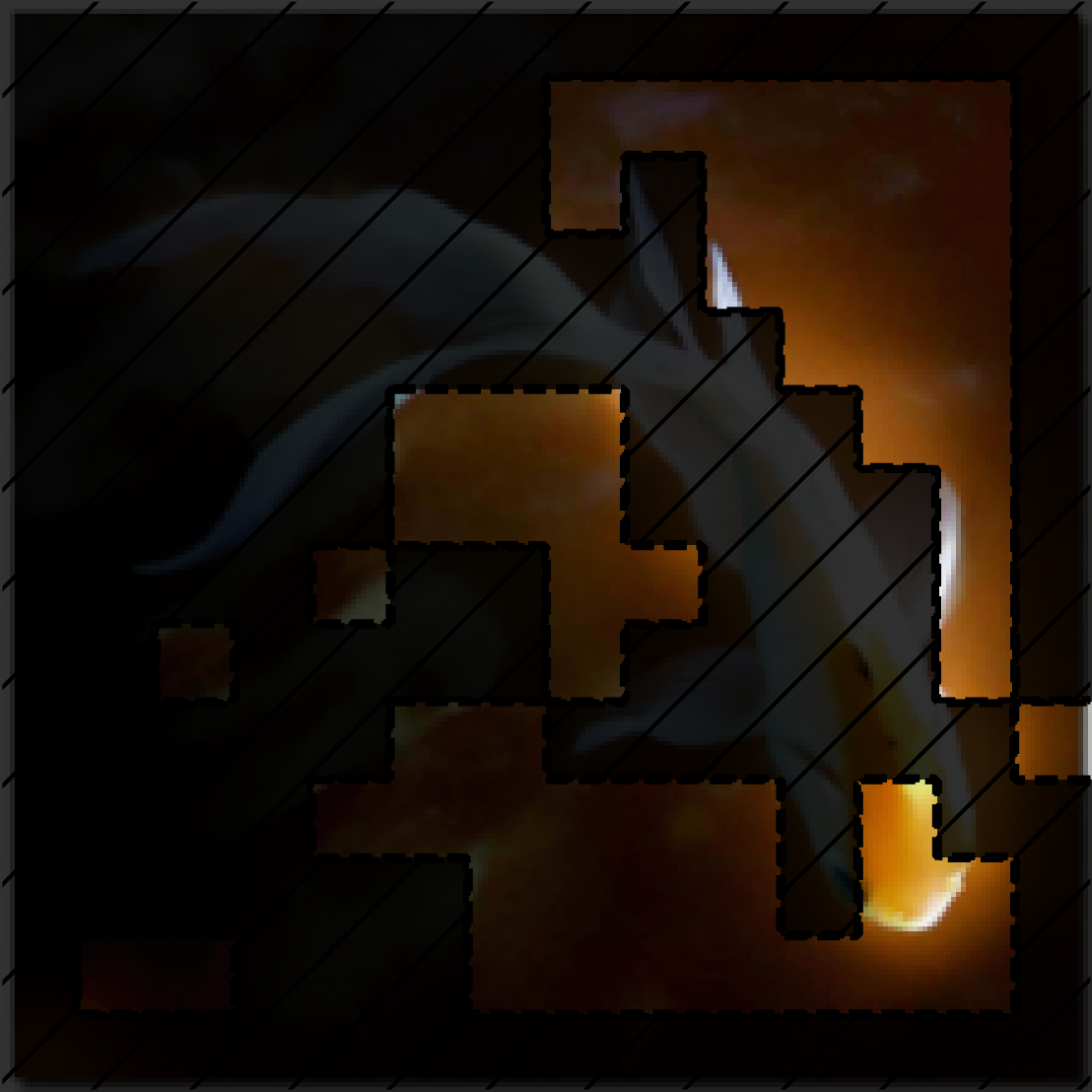

  

  2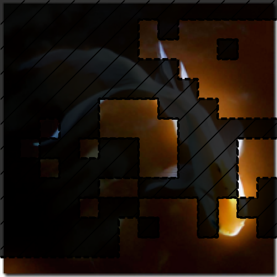

  

  Grouped attributions from SOP. The masked out areas in the images are zeroed out, and the unmasked areas are preserved features for each group. The first row shows groups that are weighted most in prediction. The second row shows groups that are weighted the least (0) in prediction. Probability for each group's predicted class is shown. Predicted classes marked blue are what is consistent with the final aggregated prediction, while red are inconsistent.

• 0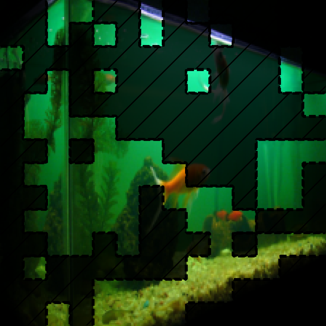

  

  1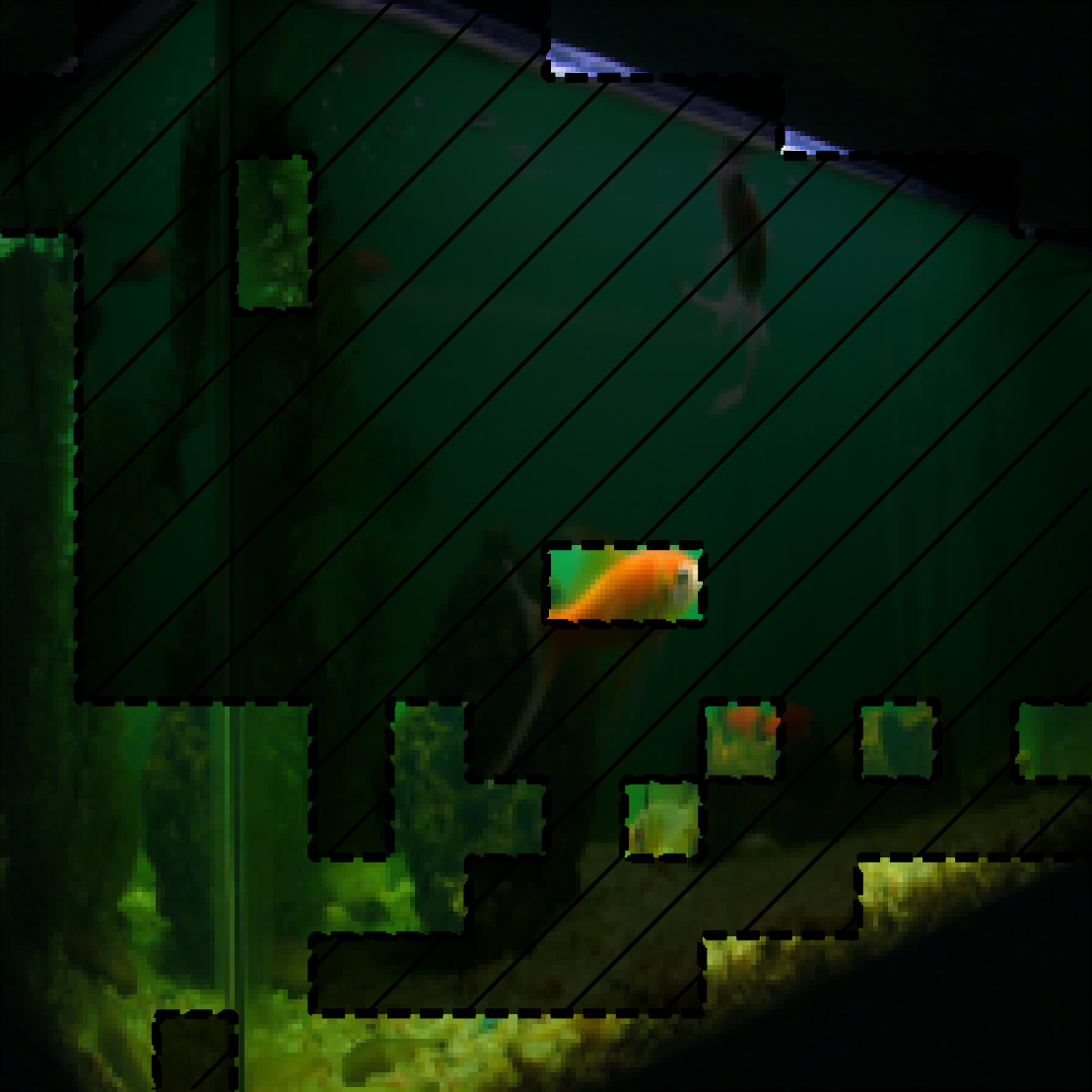

  

  2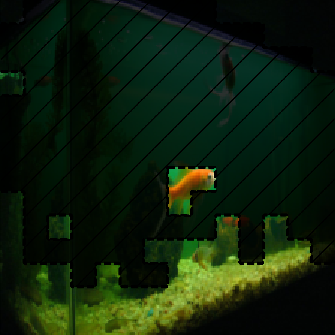

  

  0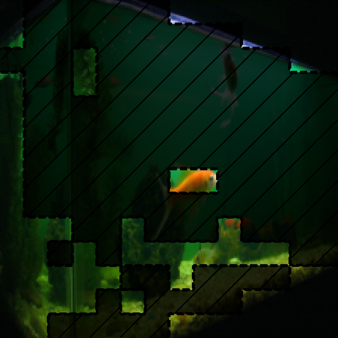

  

  1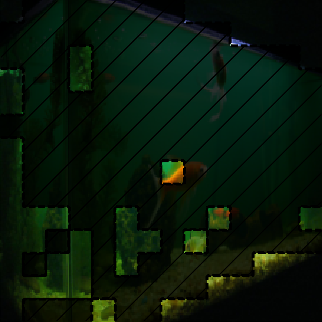

  

  2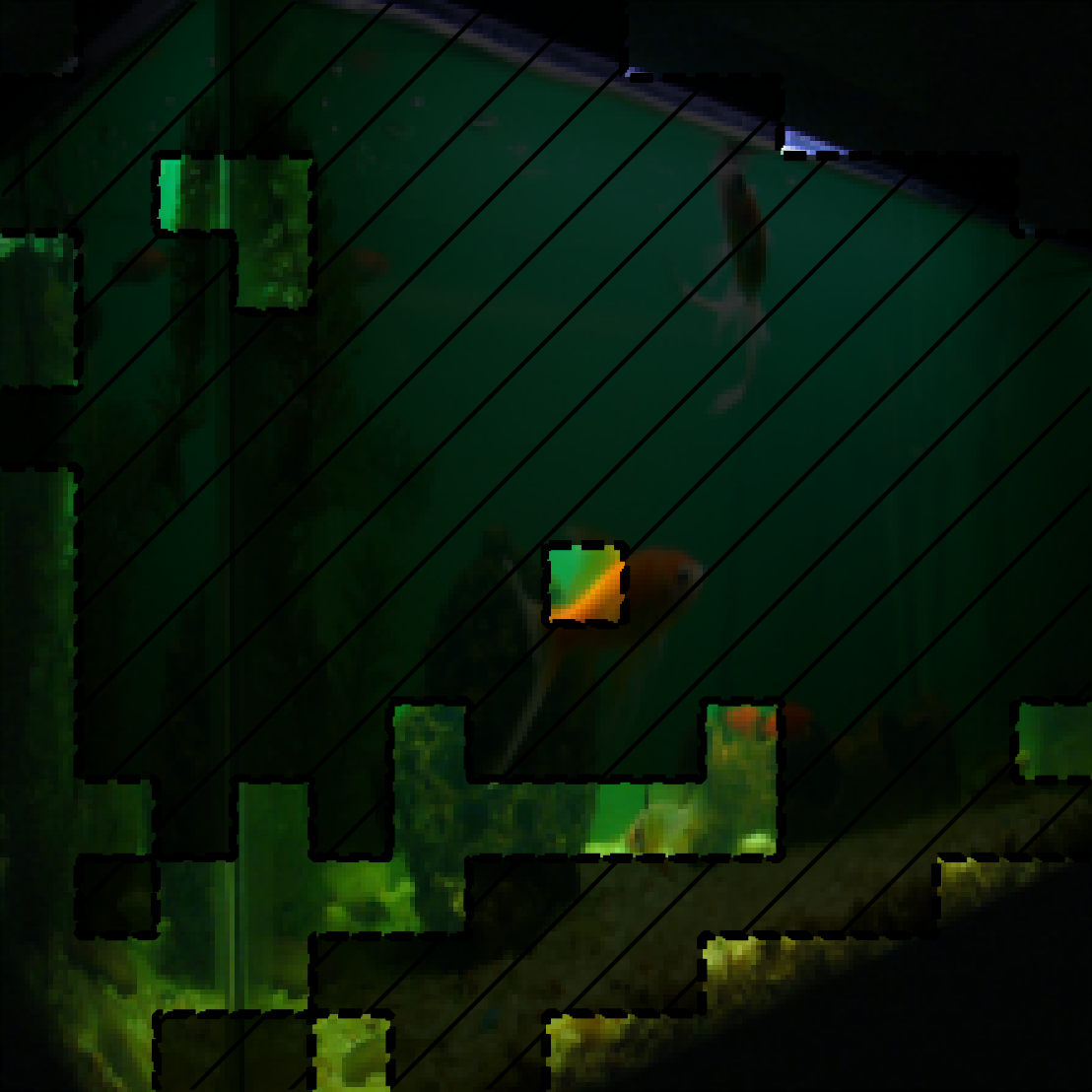

  

  Grouped attributions from SOP. The masked out areas in the images are zeroed out, and the unmasked areas are preserved features for each group. The first row shows groups that are weighted most in prediction. The second row shows groups that are weighted the least (0) in prediction. Probability for each group's predicted class is shown. Predicted classes marked blue are what is consistent with the final aggregated prediction, while red are inconsistent.

• 0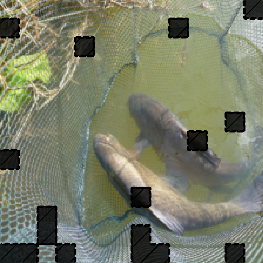

  

  1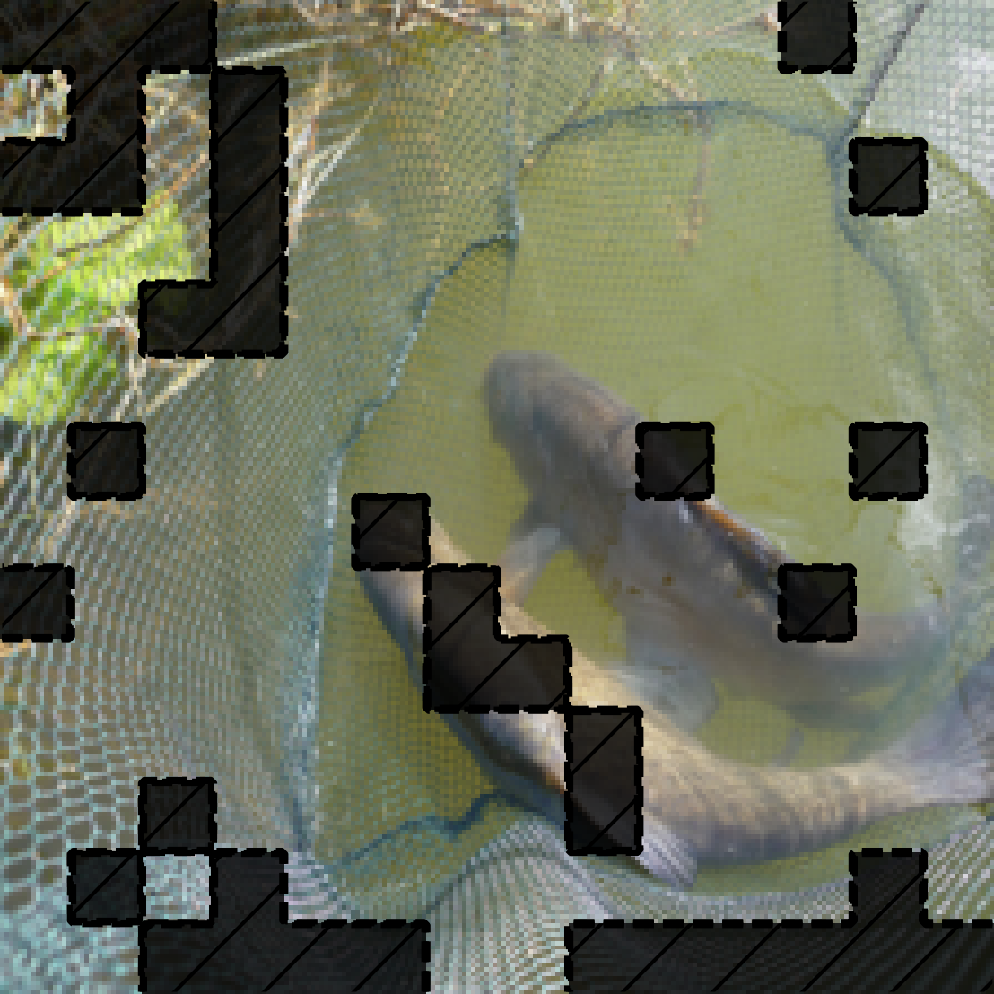

  

  2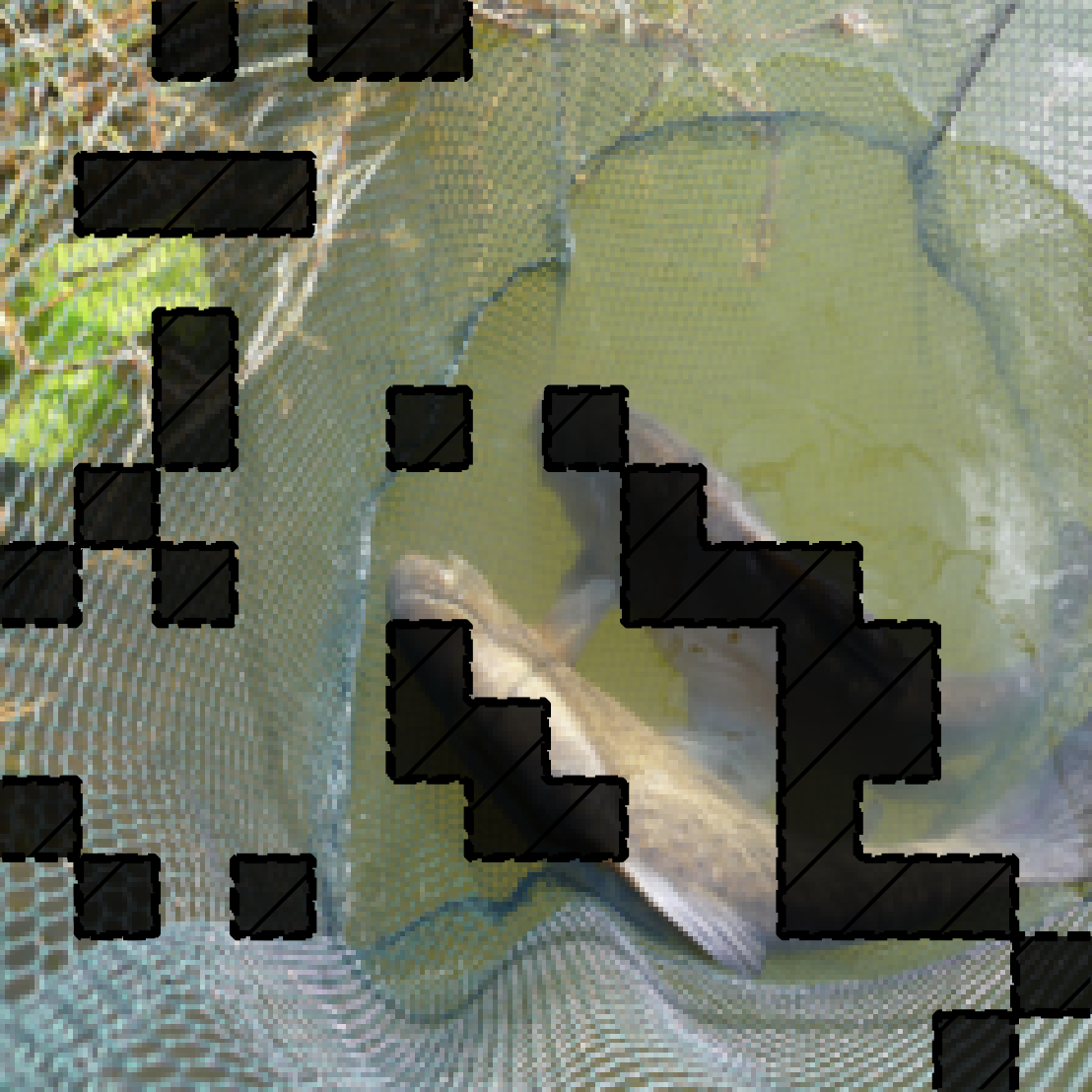

  

  0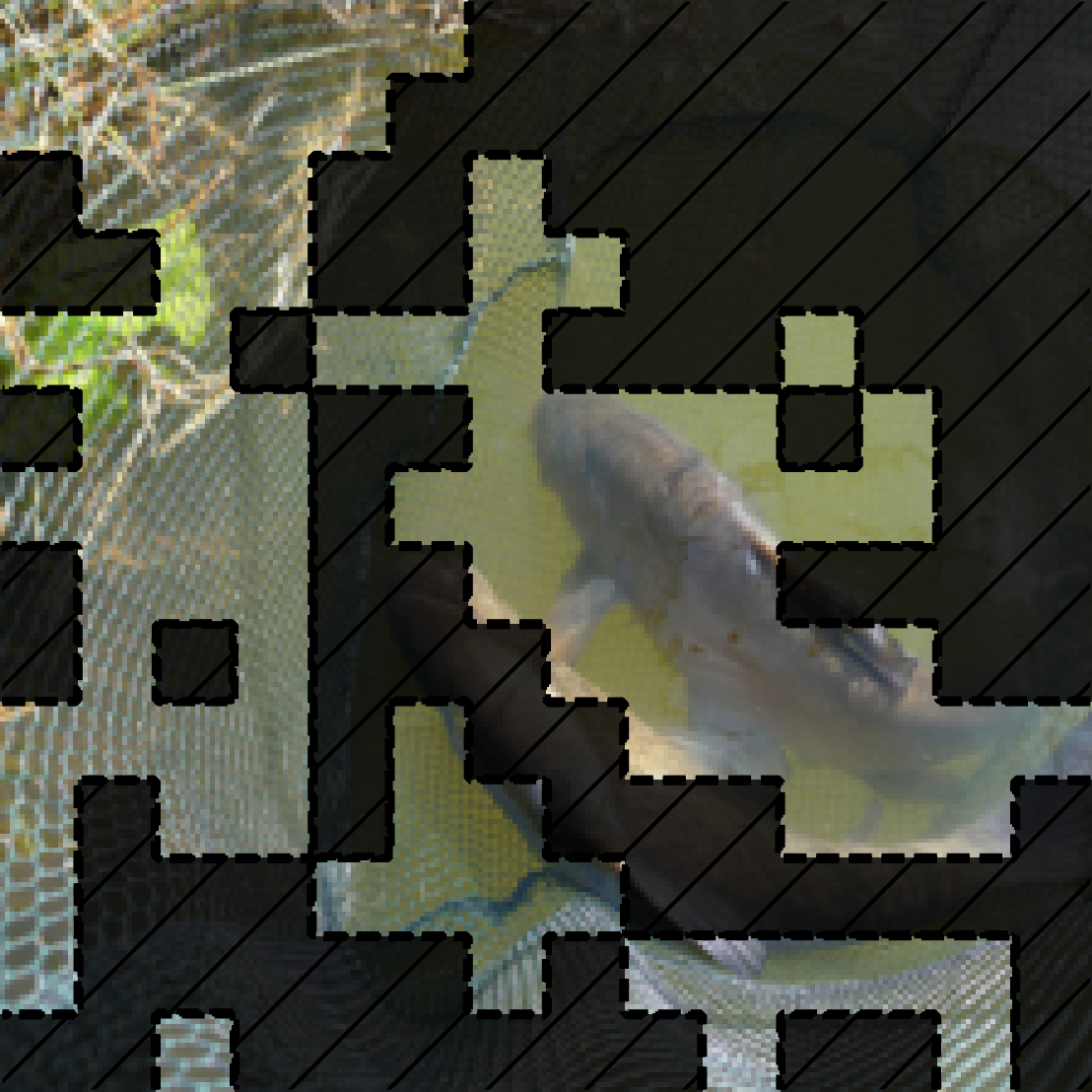

  

  1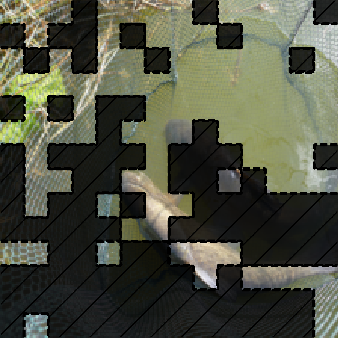

  

  2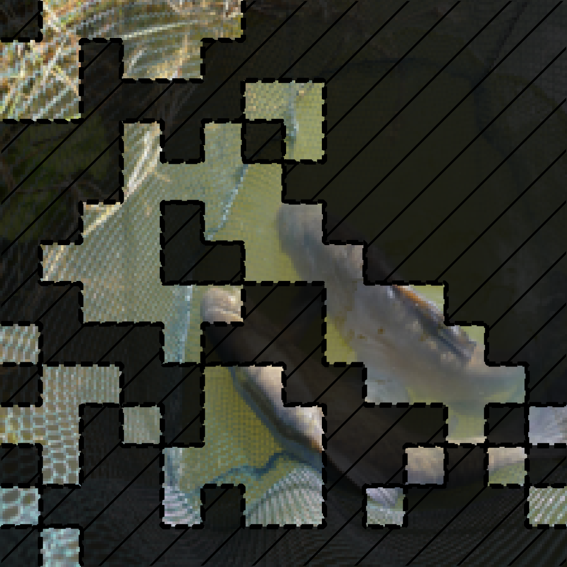

  

  Grouped attributions from SOP. The masked out areas in the images are zeroed out, and the unmasked areas are preserved features for each group. The first row shows groups that are weighted most in prediction. The second row shows groups that are weighted the least (0) in prediction. Probability for each group's predicted class is shown. Predicted classes marked blue are what is consistent with the final aggregated prediction, while red are inconsistent.

• 0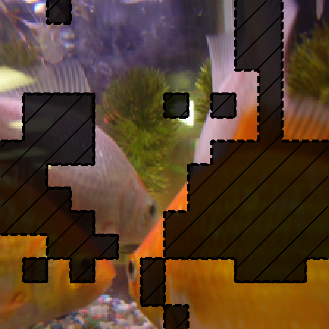

  

  1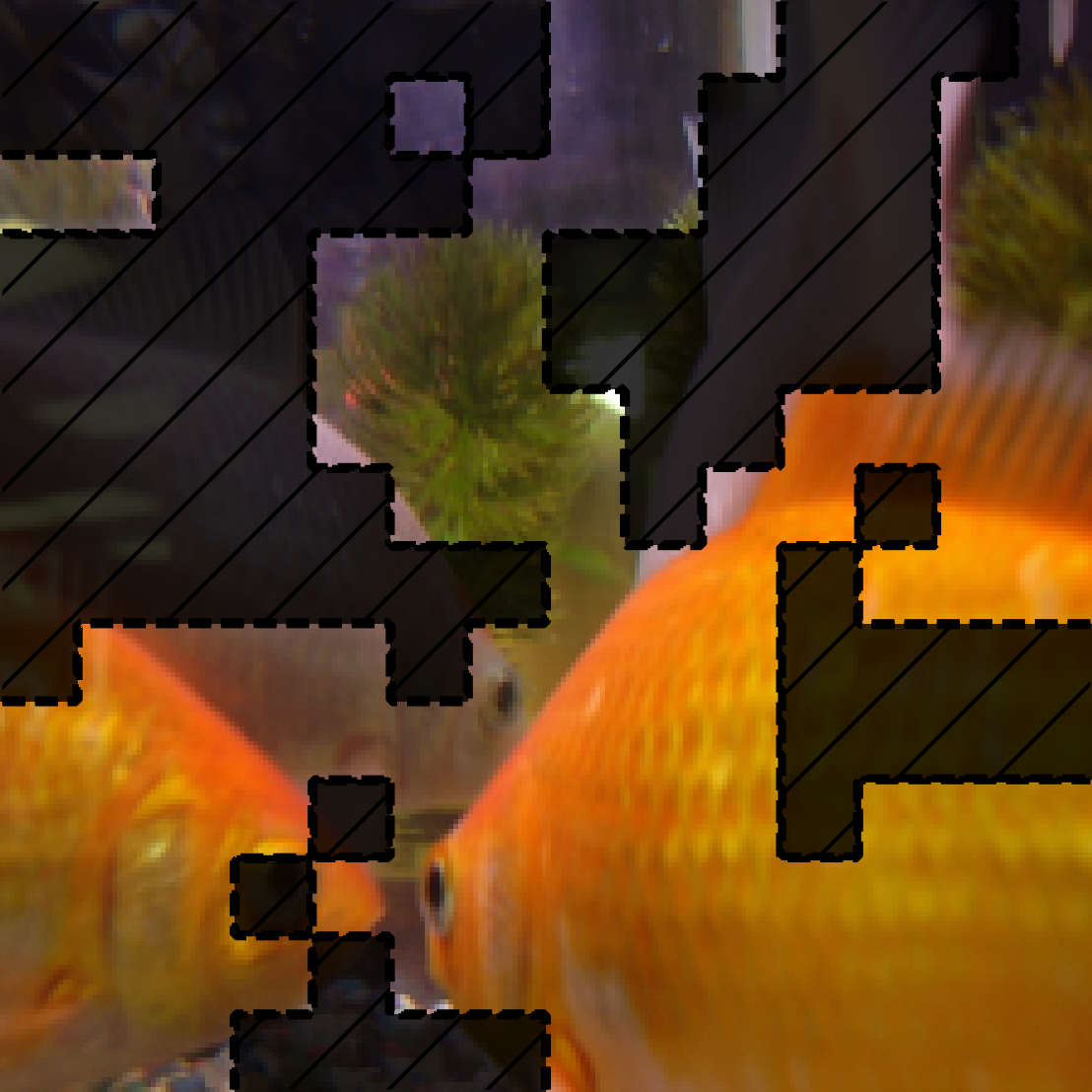

  

  2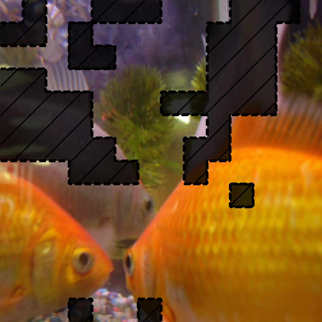

  

  0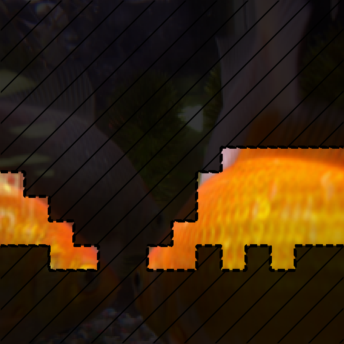

  

  1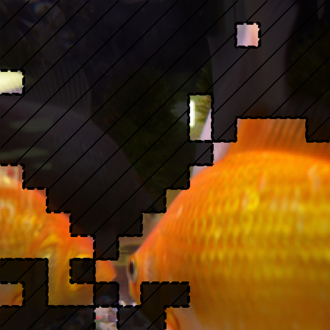

  

  2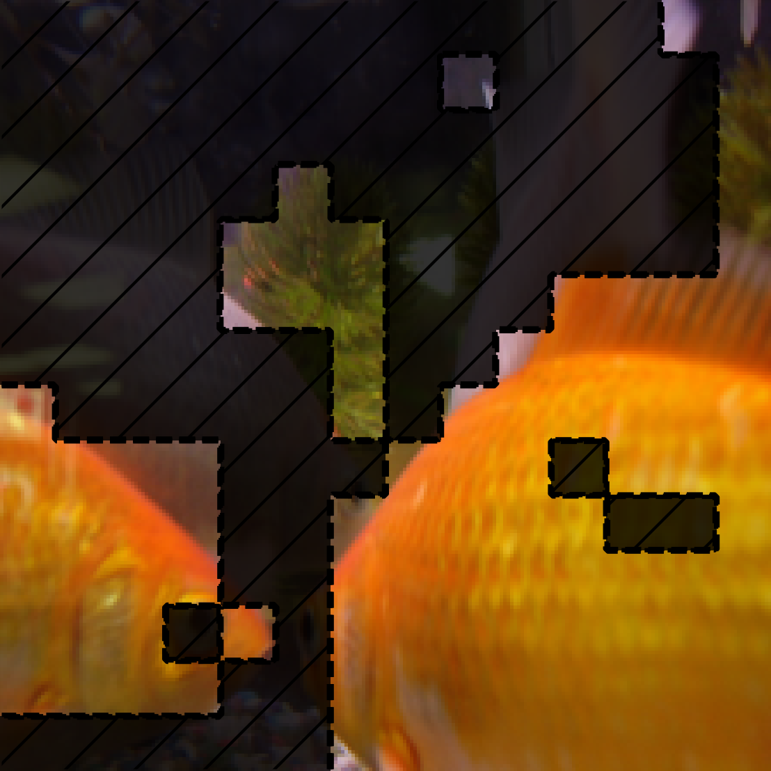

  

  Grouped attributions from SOP. The masked out areas in the images are zeroed out, and the unmasked areas are preserved features for each group. The first row shows groups that are weighted most in prediction. The second row shows groups that are weighted the least (0) in prediction. Probability for each group's predicted class is shown. Predicted classes marked blue are what is consistent with the final aggregated prediction, while red are inconsistent.

• 0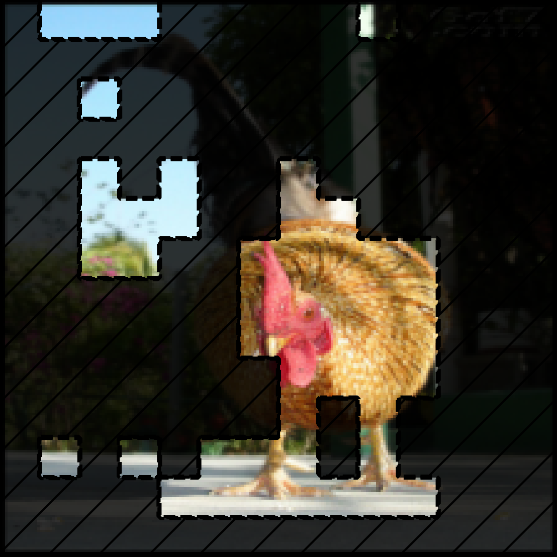

  

  1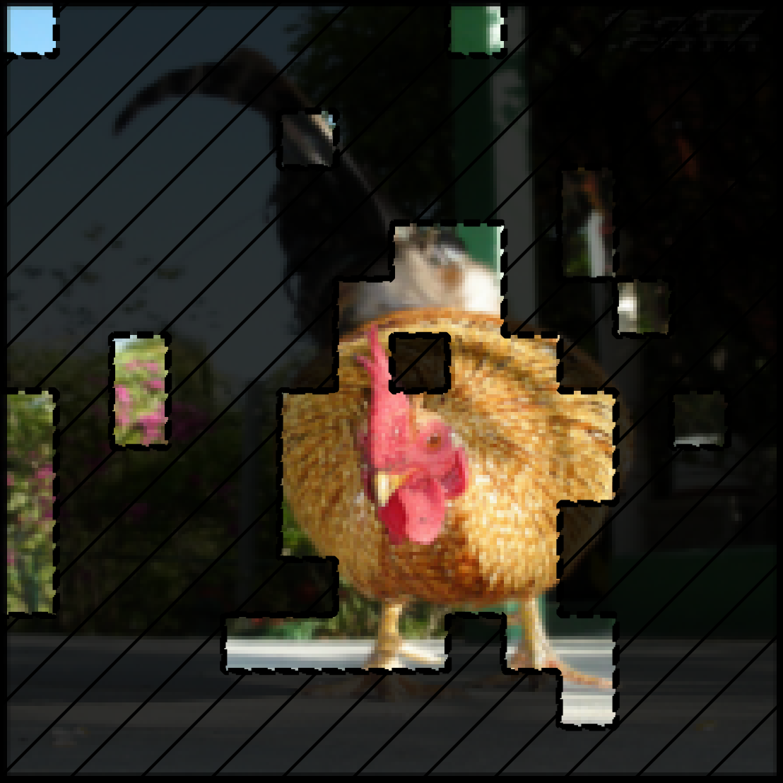

  

  2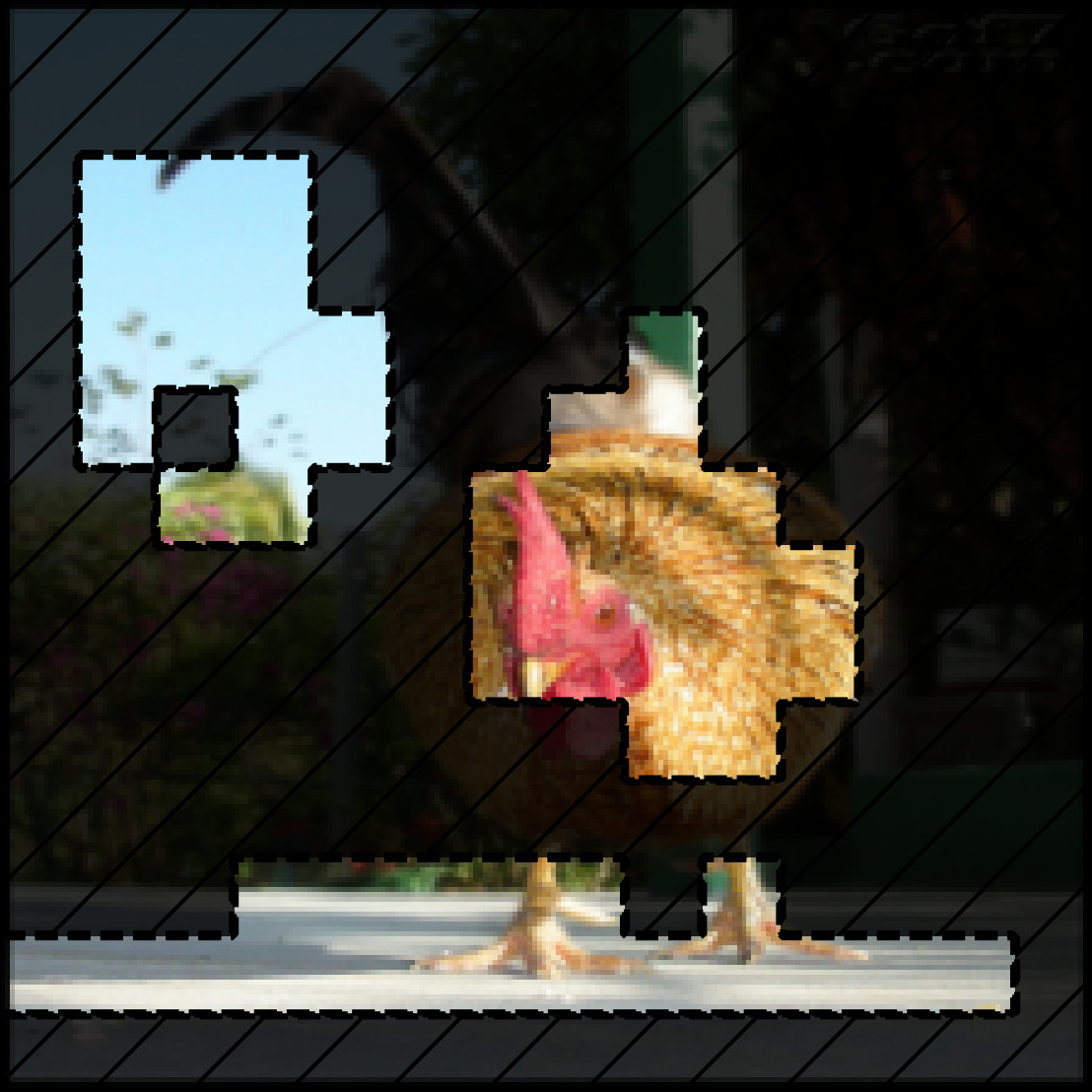

  

  0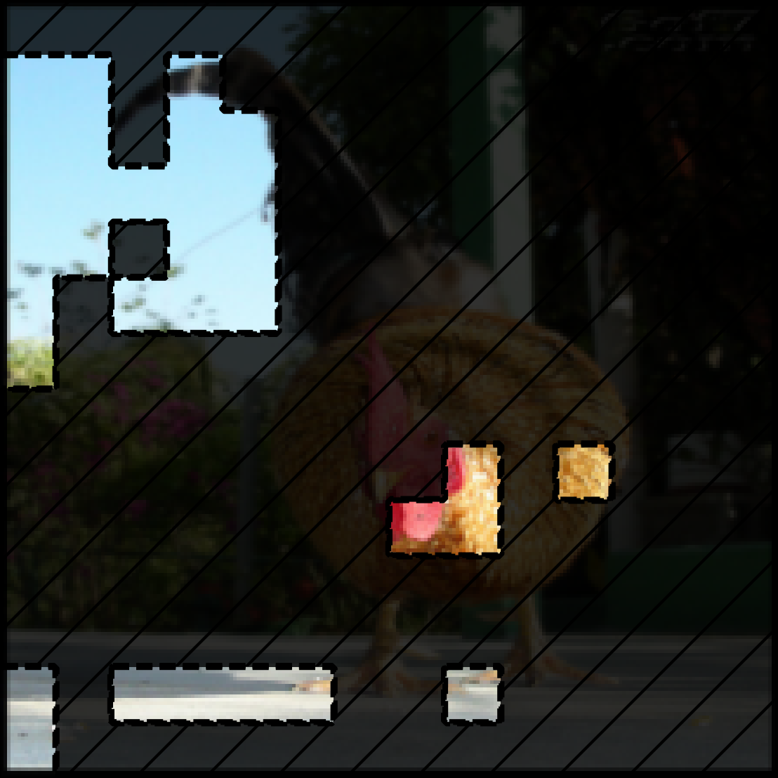

  

  1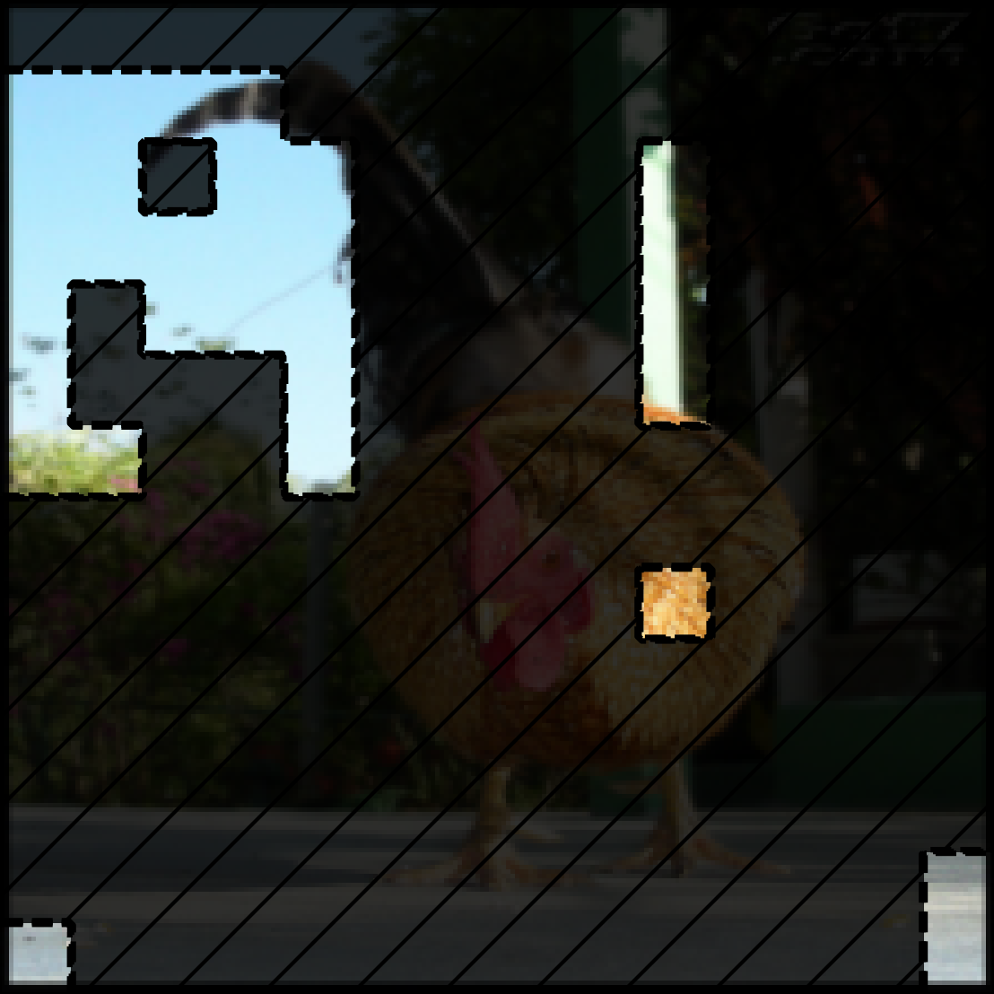

  

  2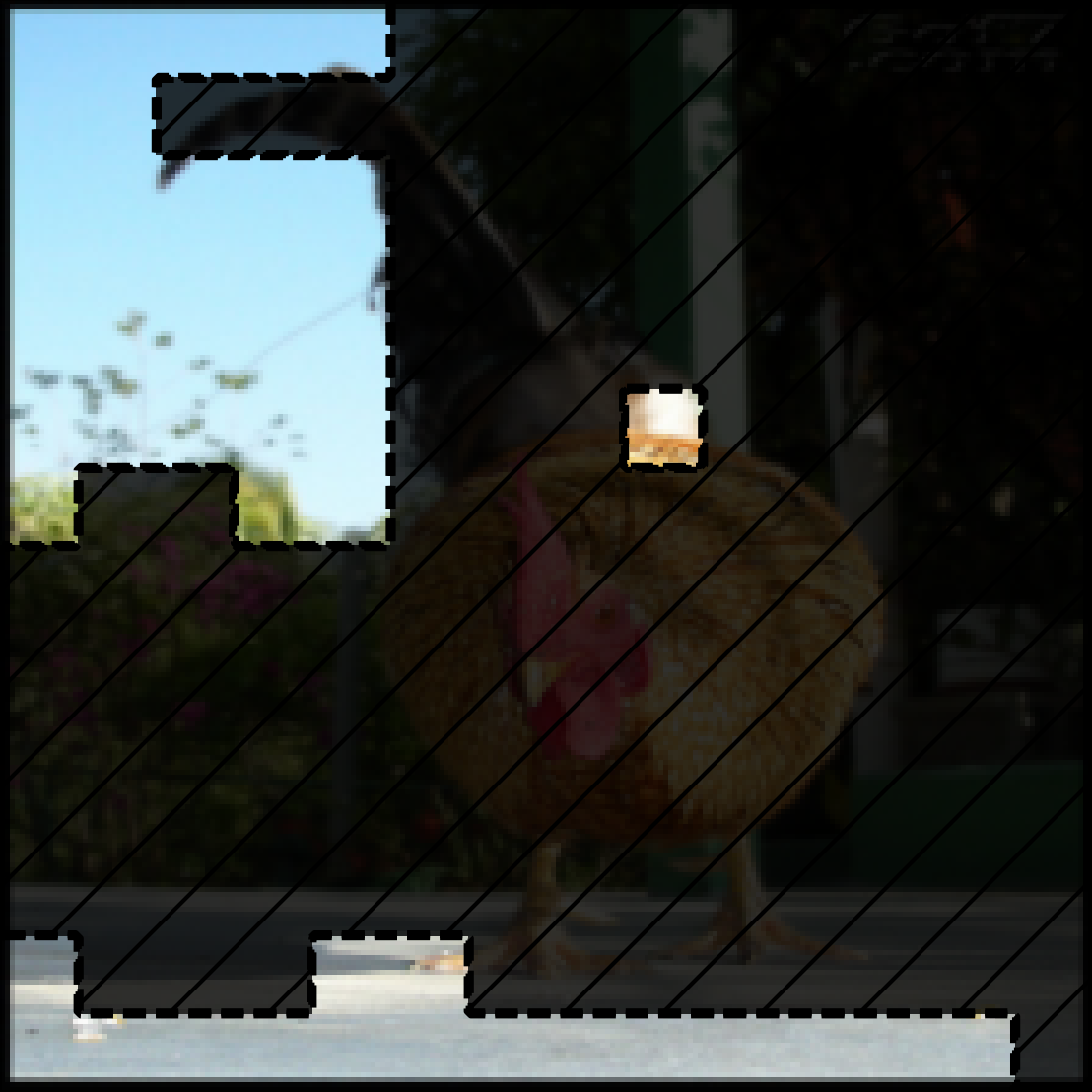

  

  Grouped attributions from SOP. The masked out areas in the images are zeroed out, and the unmasked areas are preserved features for each group. The first row shows groups that are weighted most in prediction. The second row shows groups that are weighted the least (0) in prediction. Probability for each group's predicted class is shown. Predicted classes marked blue are what is consistent with the final aggregated prediction, while red are inconsistent.

• 0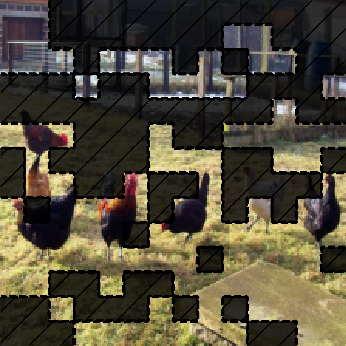

  

  1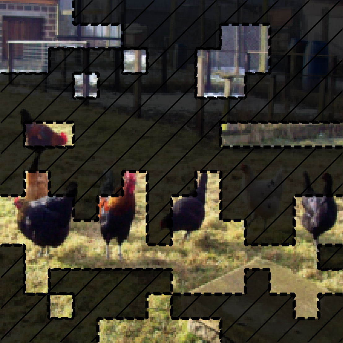

  

  2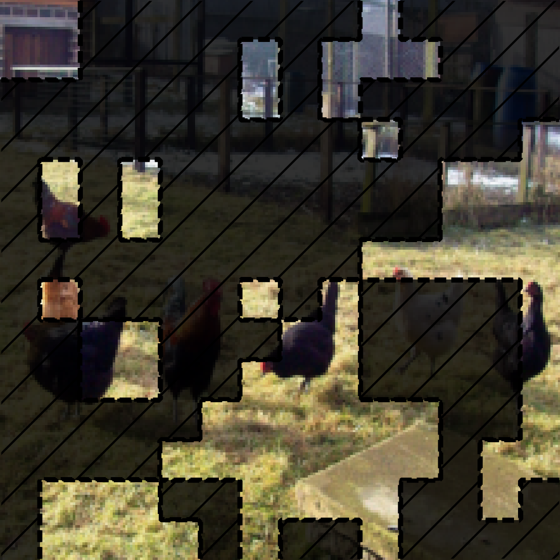

  

  0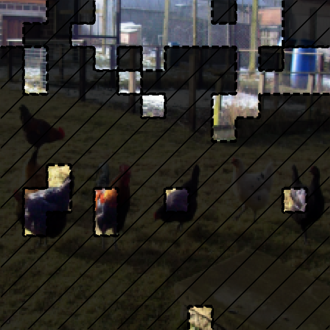

  

  1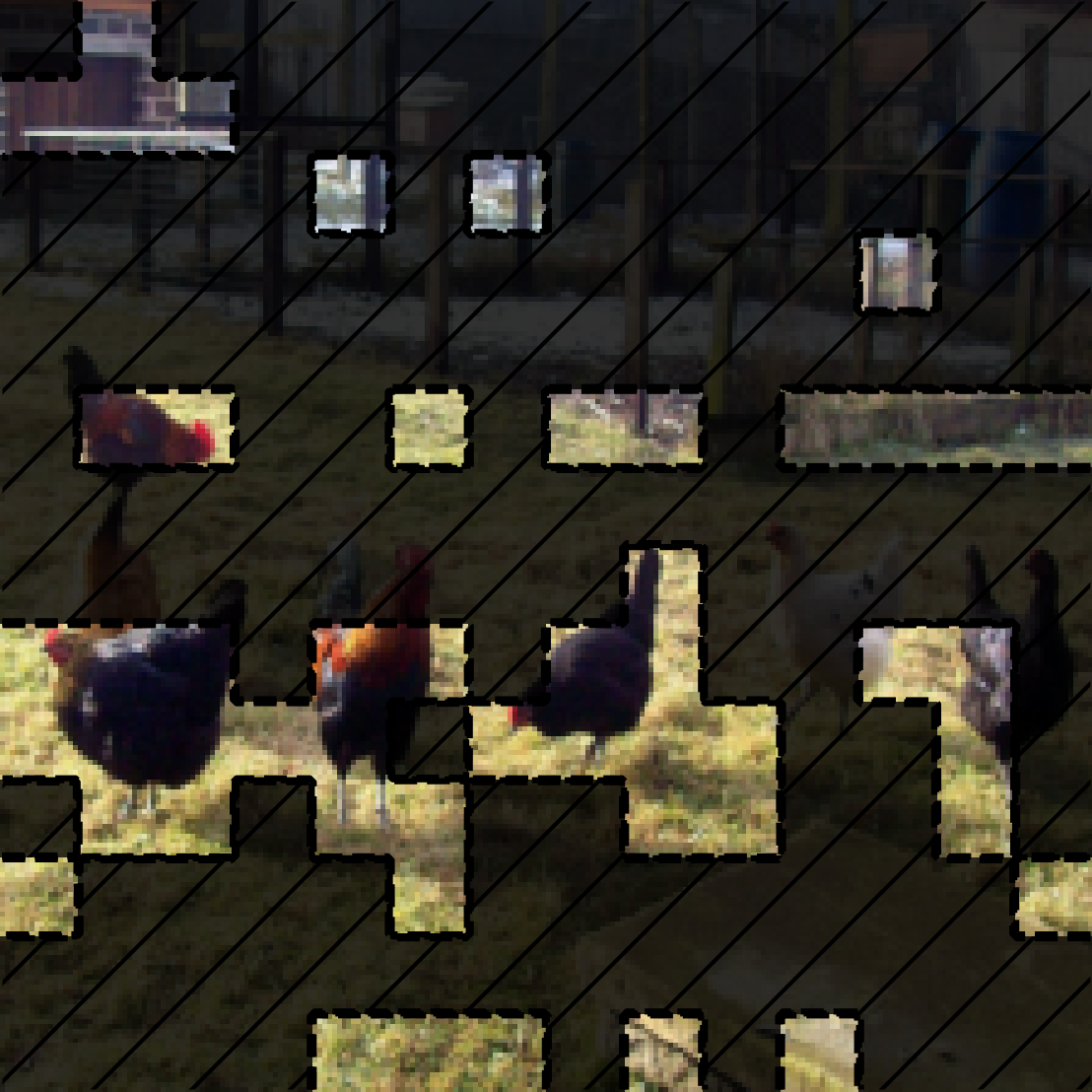

  

  2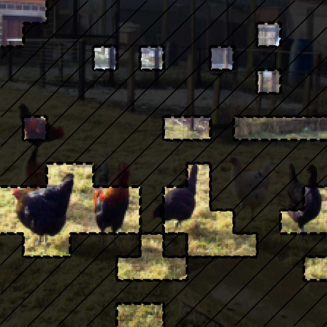

  

  Grouped attributions from SOP. The masked out areas in the images are zeroed out, and the unmasked areas are preserved features for each group. The first row shows groups that are weighted most in prediction. The second row shows groups that are weighted the least (0) in prediction. Probability for each group's predicted class is shown. Predicted classes marked blue are what is consistent with the final aggregated prediction, while red are inconsistent.

• 0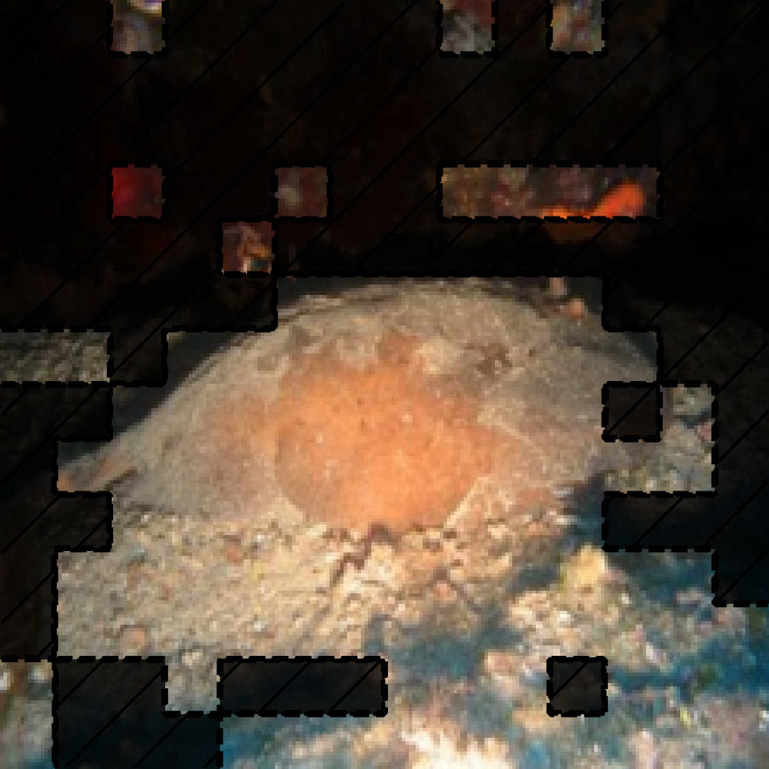

  

  1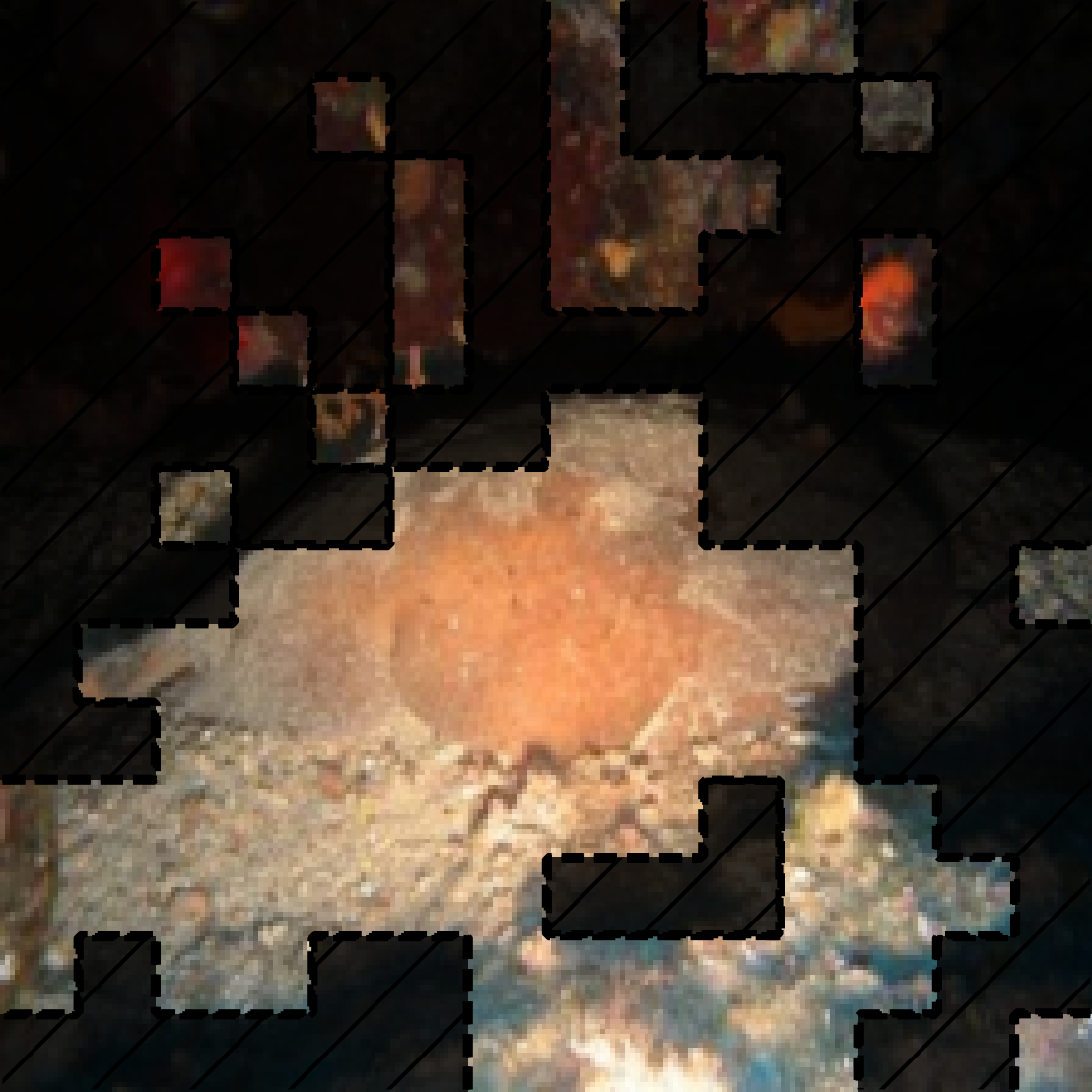

  

  2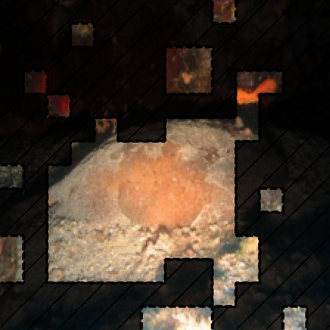

  

  0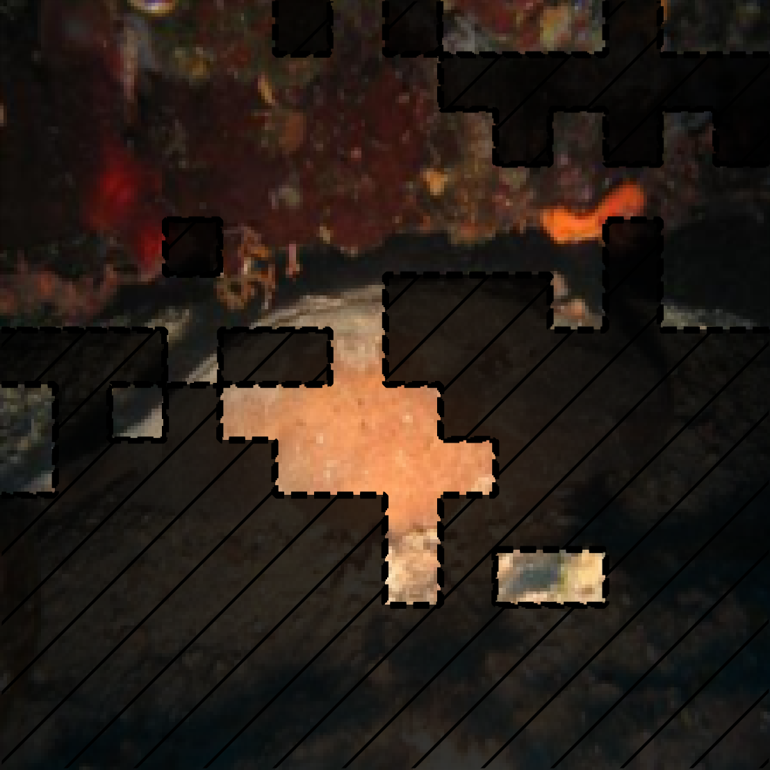

  

  1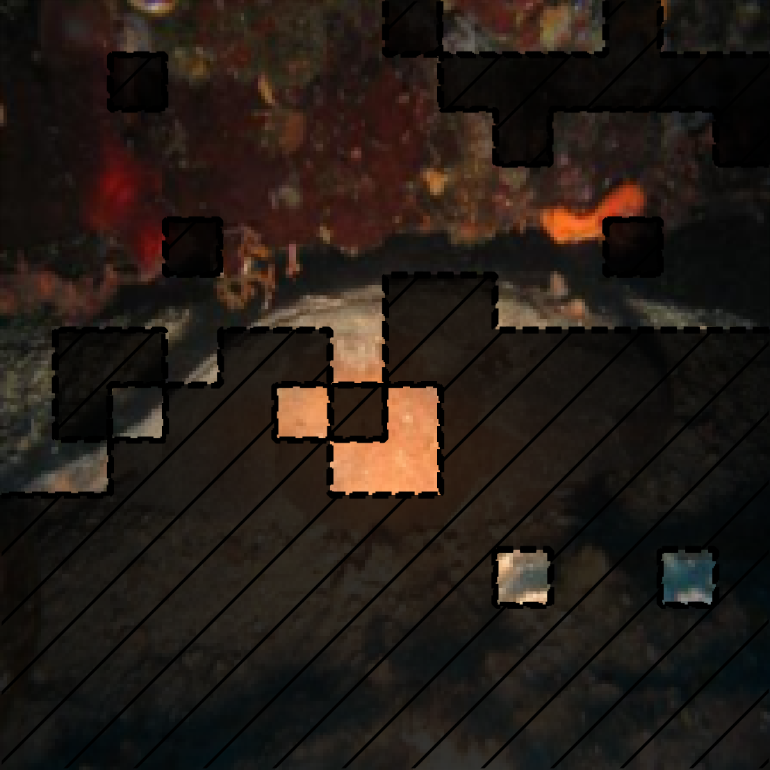

  

  2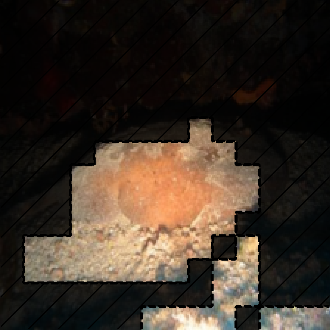

  

  Grouped attributions from SOP. The masked out areas in the images are zeroed out, and the unmasked areas are preserved features for each group. The first row shows groups that are weighted most in prediction. The second row shows groups that are weighted the least (0) in prediction. Probability for each group's predicted class is shown. Predicted classes marked blue are what is consistent with the final aggregated prediction, while red are inconsistent.

• 0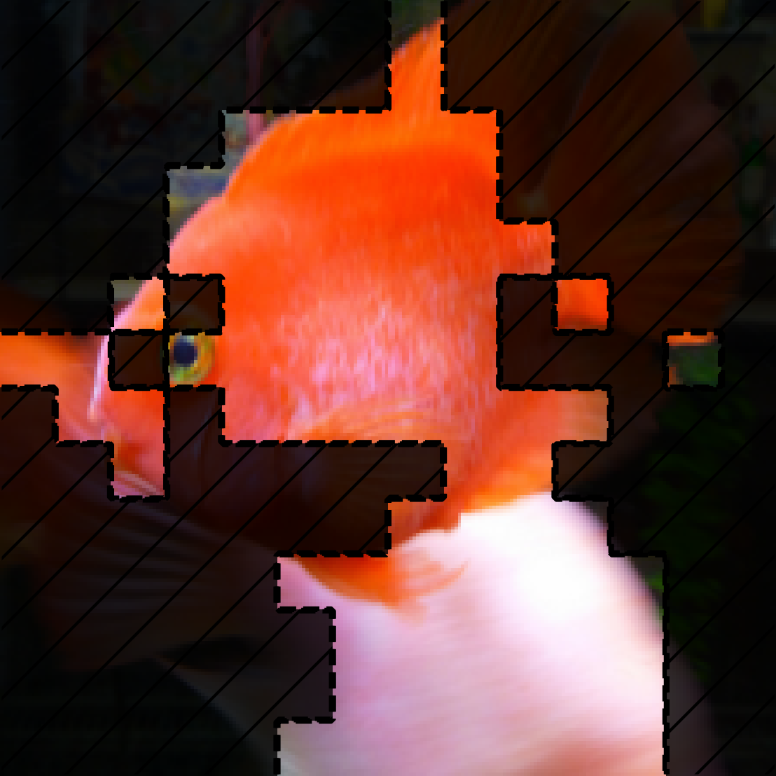

  

  1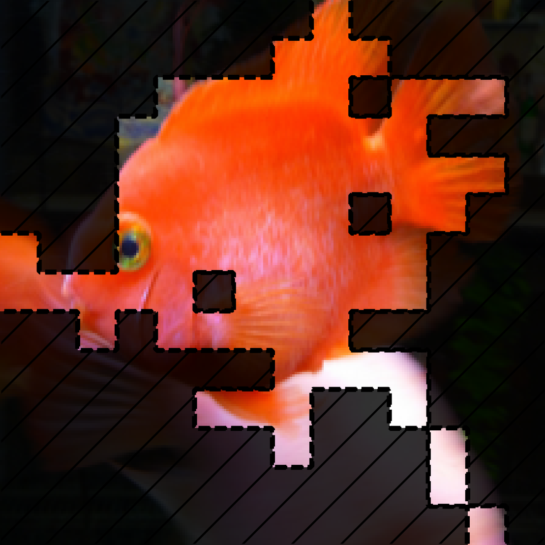

  

  2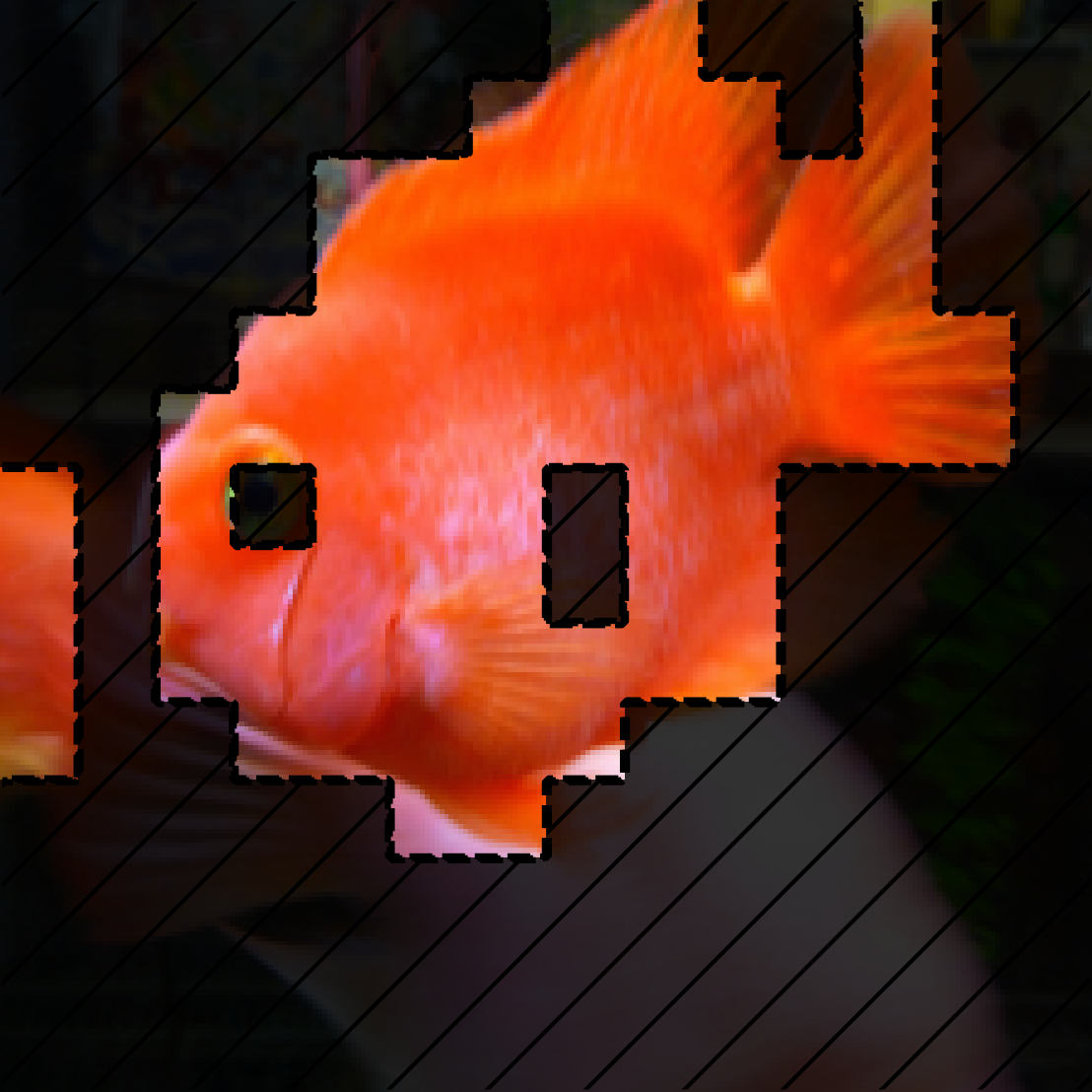

  

  0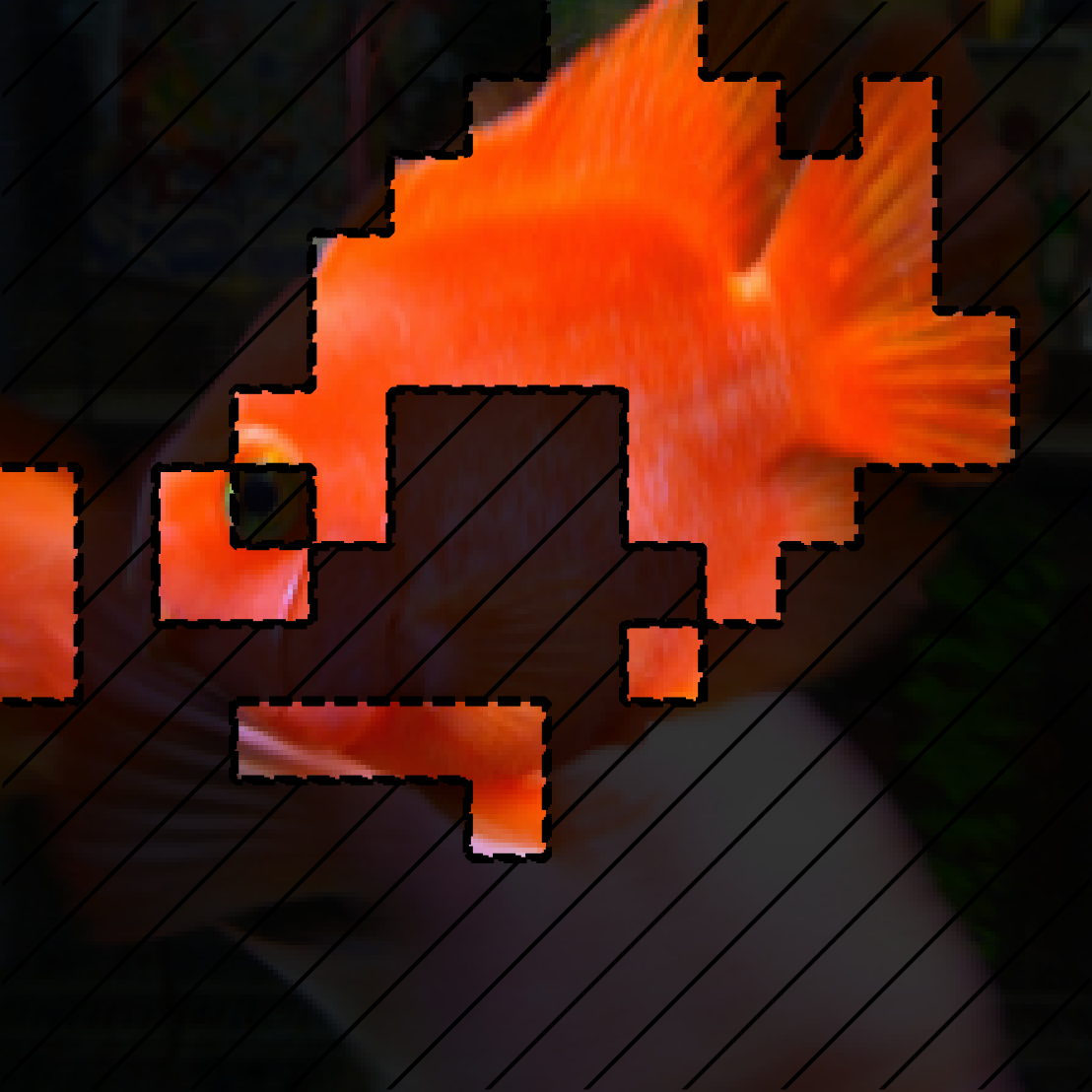

  

  1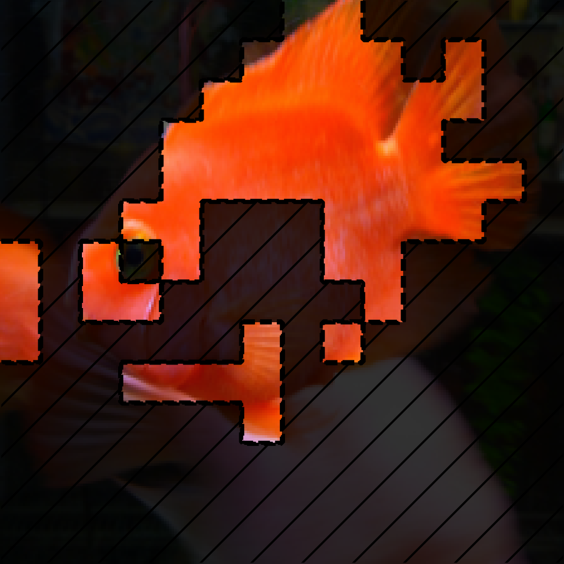

  

  2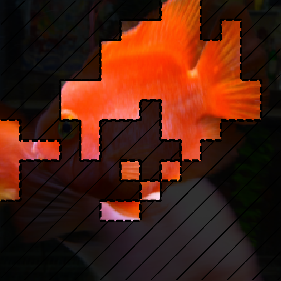

  

  Grouped attributions from SOP. The masked out areas in the images are zeroed out, and the unmasked areas are preserved features for each group. The first row shows groups that are weighted most in prediction. The second row shows groups that are weighted the least (0) in prediction. Probability for each group's predicted class is shown. Predicted classes marked blue are what is consistent with the final aggregated prediction, while red are inconsistent.

• 0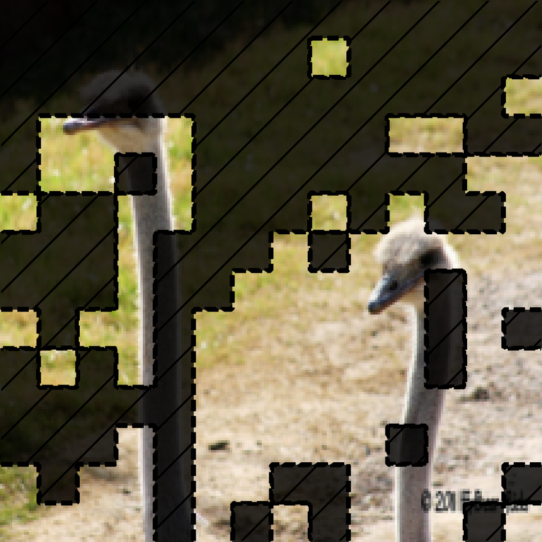

  

  1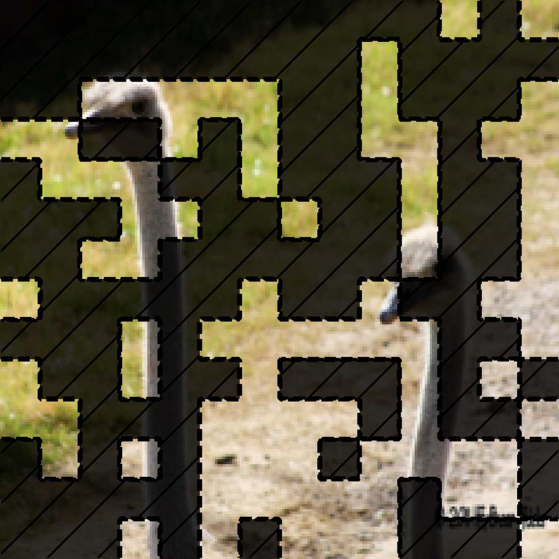

  

  2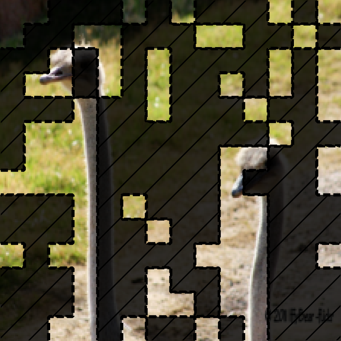

  

  0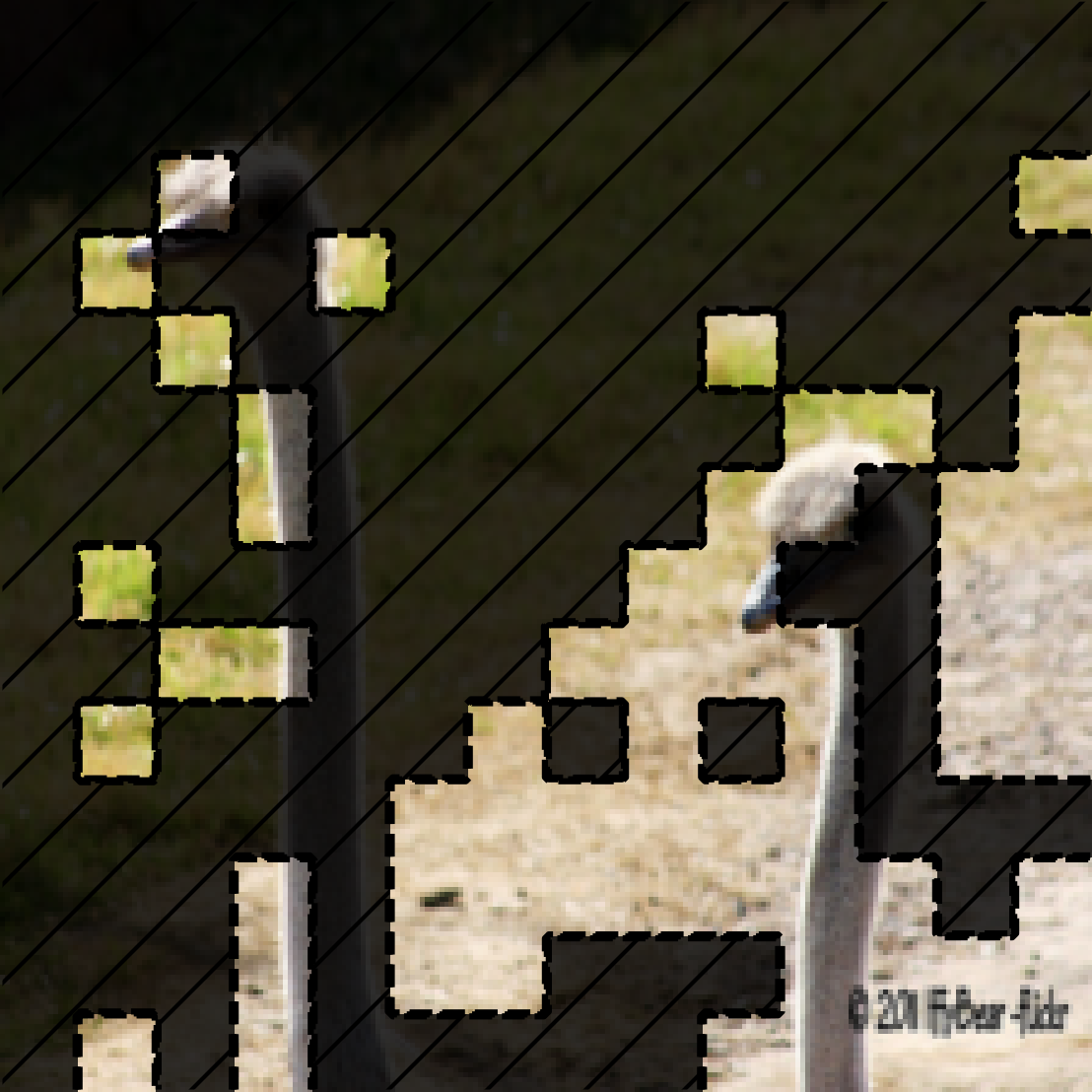

  

  1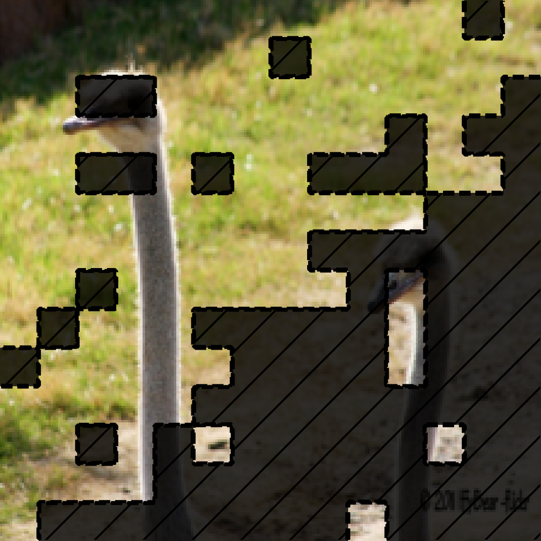

  

  2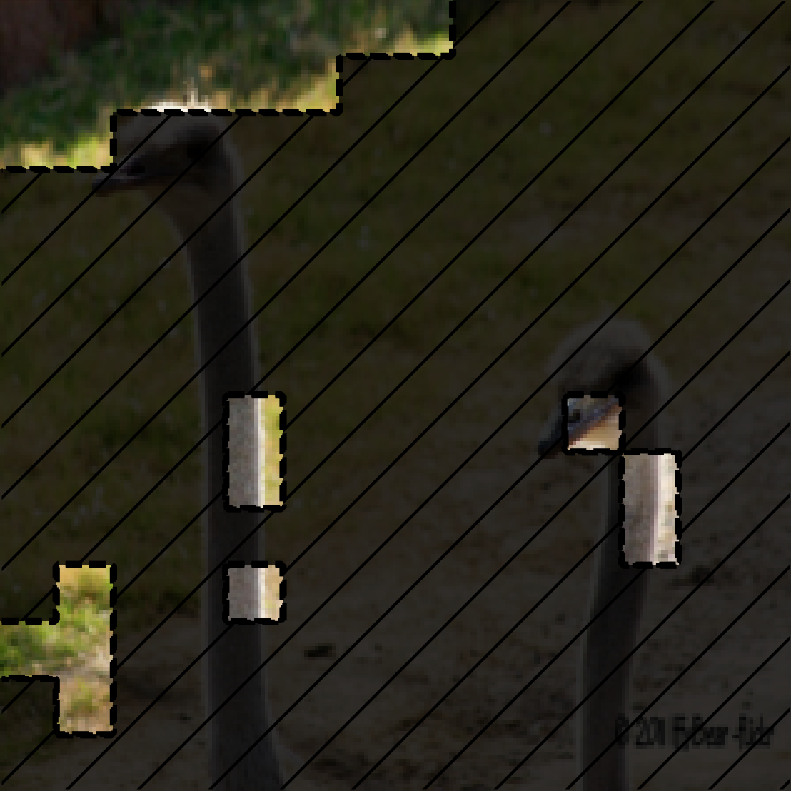

  

  Grouped attributions from SOP. The masked out areas in the images are zeroed out, and the unmasked areas are preserved features for each group. The first row shows groups that are weighted most in prediction. The second row shows groups that are weighted the least (0) in prediction. Probability for each group's predicted class is shown. Predicted classes marked blue are what is consistent with the final aggregated prediction, while red are inconsistent.

• 0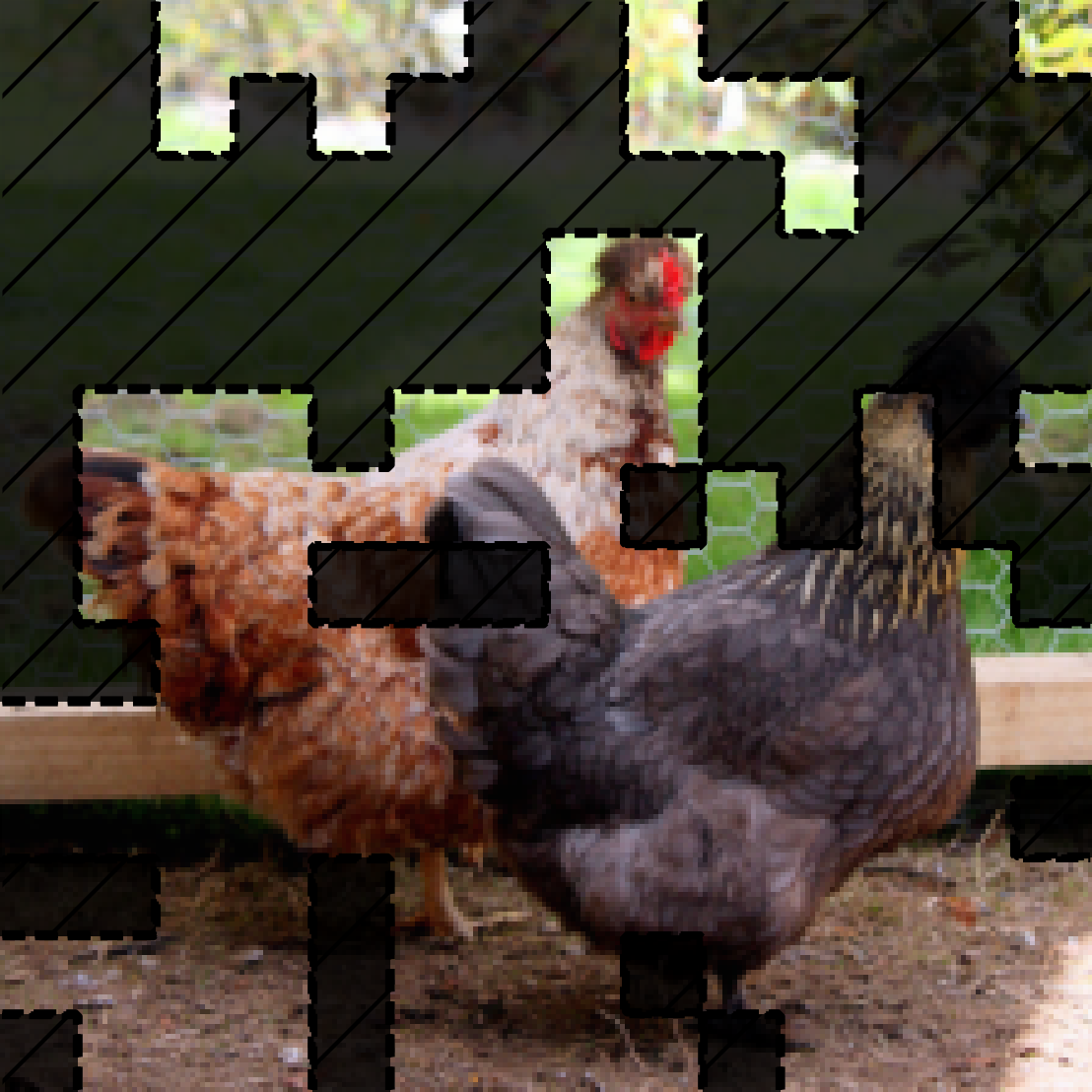

  

  1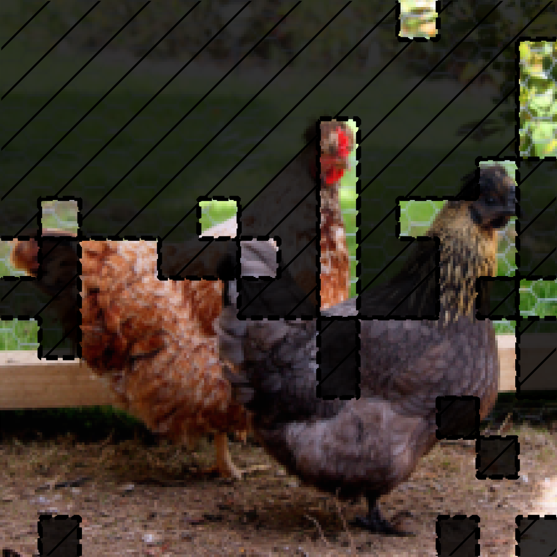

  

  2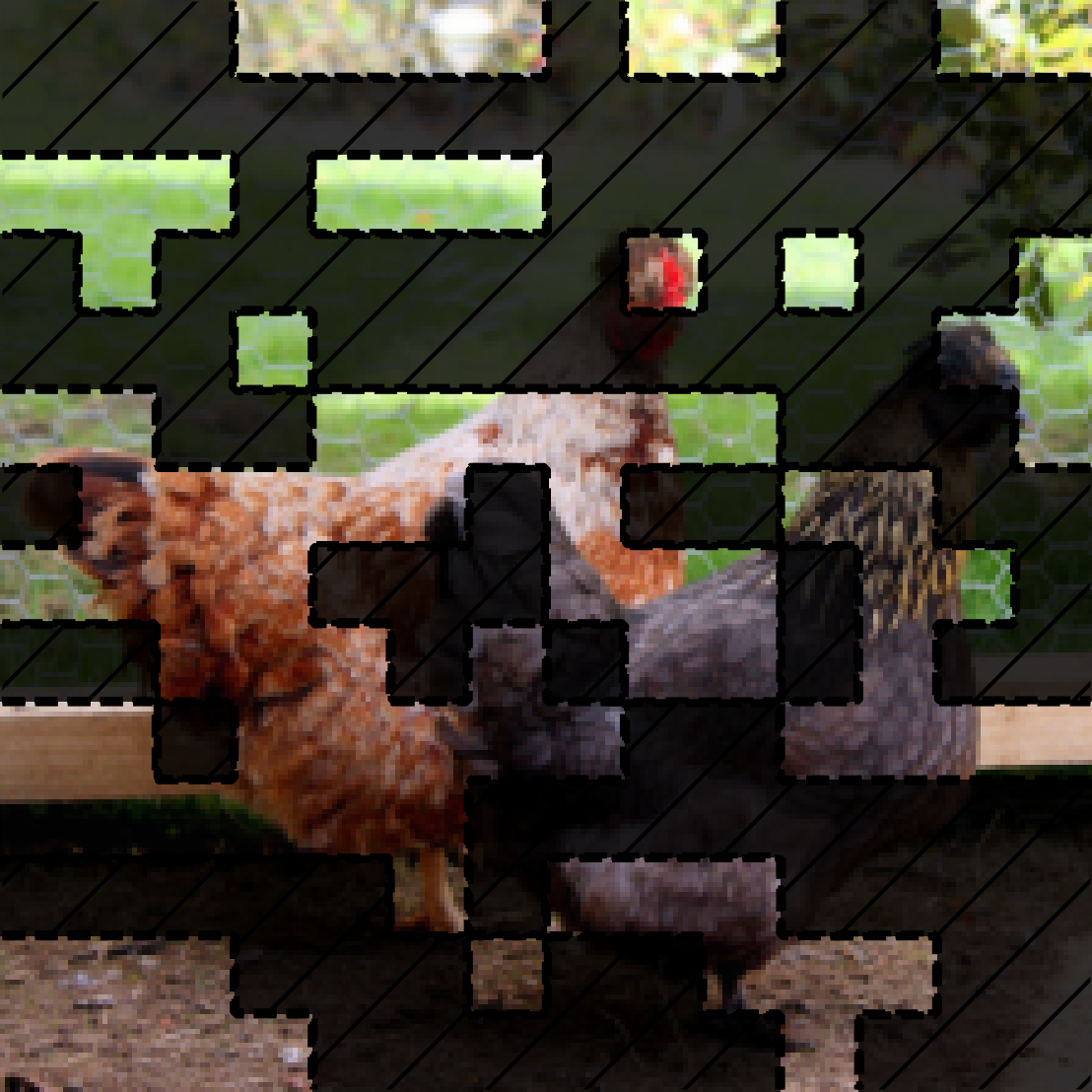

  

  0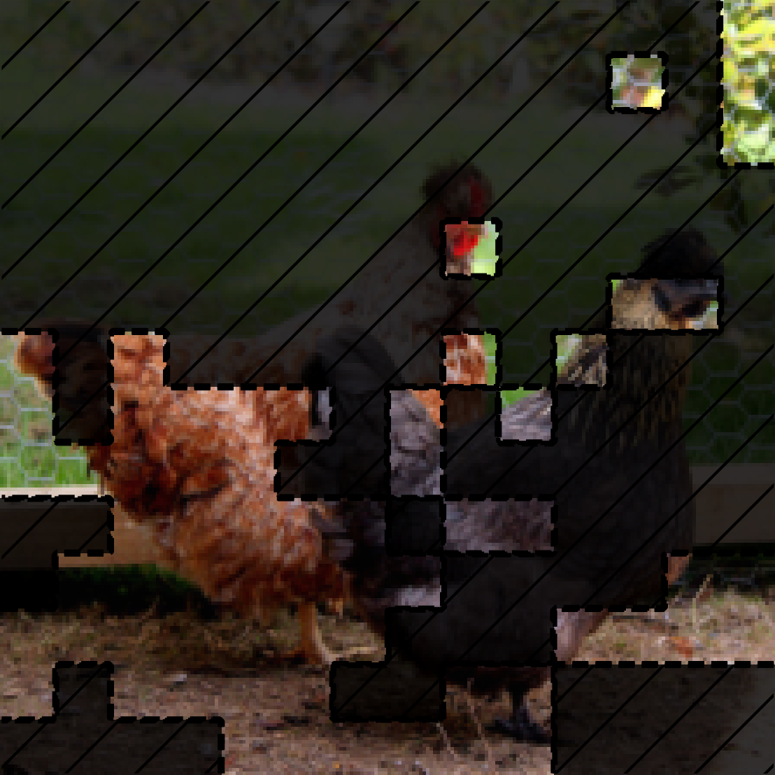

  

  1

  

  2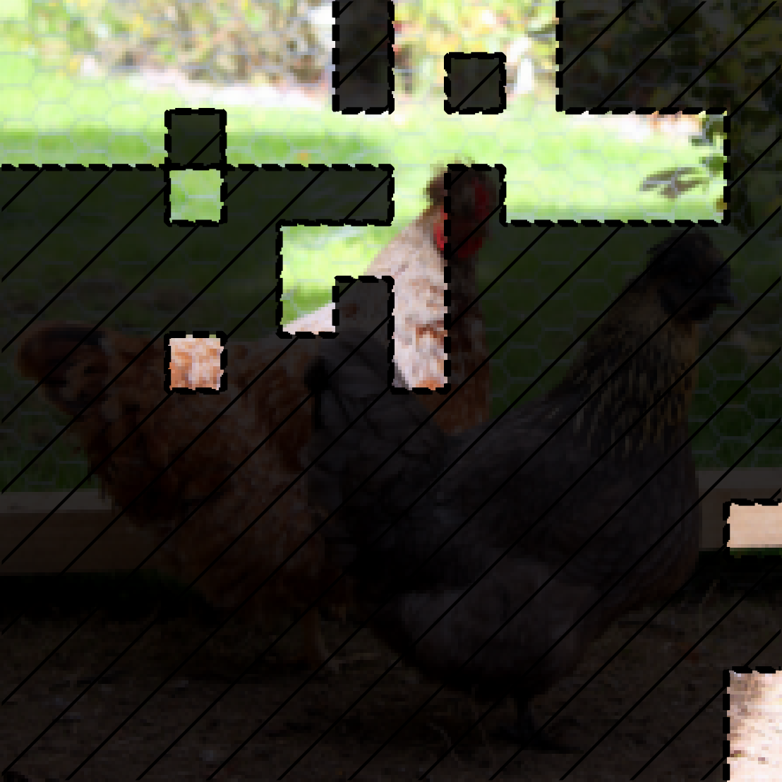

  

  Grouped attributions from SOP. The masked out areas in the images are zeroed out, and the unmasked areas are preserved features for each group. The first row shows groups that are weighted most in prediction. The second row shows groups that are weighted the least (0) in prediction. Probability for each group's predicted class is shown. Predicted classes marked blue are what is consistent with the final aggregated prediction, while red are inconsistent.

We can see that, for example, the second and third groups for goldfish contain most of the goldfish’s body, and they together contribute more (0.185 + 0.1554) for goldfish class than the first group which contributes 0.3398 for predicting hen.

Case Study: Cosmology

To validate the usability of our approach for solving real problems, we collaborated with cosmologists to see if we could use the groups for scientific discovery.

Weak lensing maps in cosmology calculate the spatial distribution of matter density in the universe (Gatti et al. 2021). Cosmologists hope to use weak lensing maps to predict two key parameters related to the initial state of the universe: $\Omega_m$ and $\sigma_8$.

$\Omega_m$ captures the average energy density of all matter in the universe (such as radiation and dark energy), while $\sigma_8$ describes the fluctuation of this density.

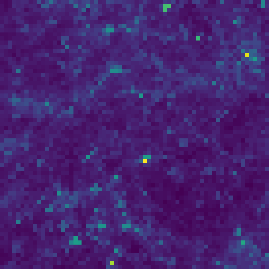
Here is an example weak lensing map:

Example of a weak lensing map. This map has $\Omega_m = 0.1021$ and $\sigma_8 = 1.023$. The large area being dark matches the low $\Omega_m$.

Matilla et al. (2020) and Ribli et al. (2019) have developed CNN models to predict $\Omega_m$ and $\sigma_8$ from simulated weak lensing maps CosmoGridV1. Even though these models have high performance, we do not fully understand how they predict $\Omega_m$ and $\sigma_8$. We then ask a question:

What groups from weak lensing maps can we use to infer $\Omega_m$ and $\sigma_8$?

We then use SOP on the trained CNN model and analyze the groups from the attributions.

The groups found by SOP are related to two types of important cosmological structures: voids and clusters. Voids are large regions that are under-dense and appear as dark regions in the weak lensing map, whereas clusters are areas of concentrated high density and appear as bright dots.

Voids

Clusters

The grayed out areas are unselected features for the group. The colored areas are preserved features, which correspond to voids (left) and clusters (right).

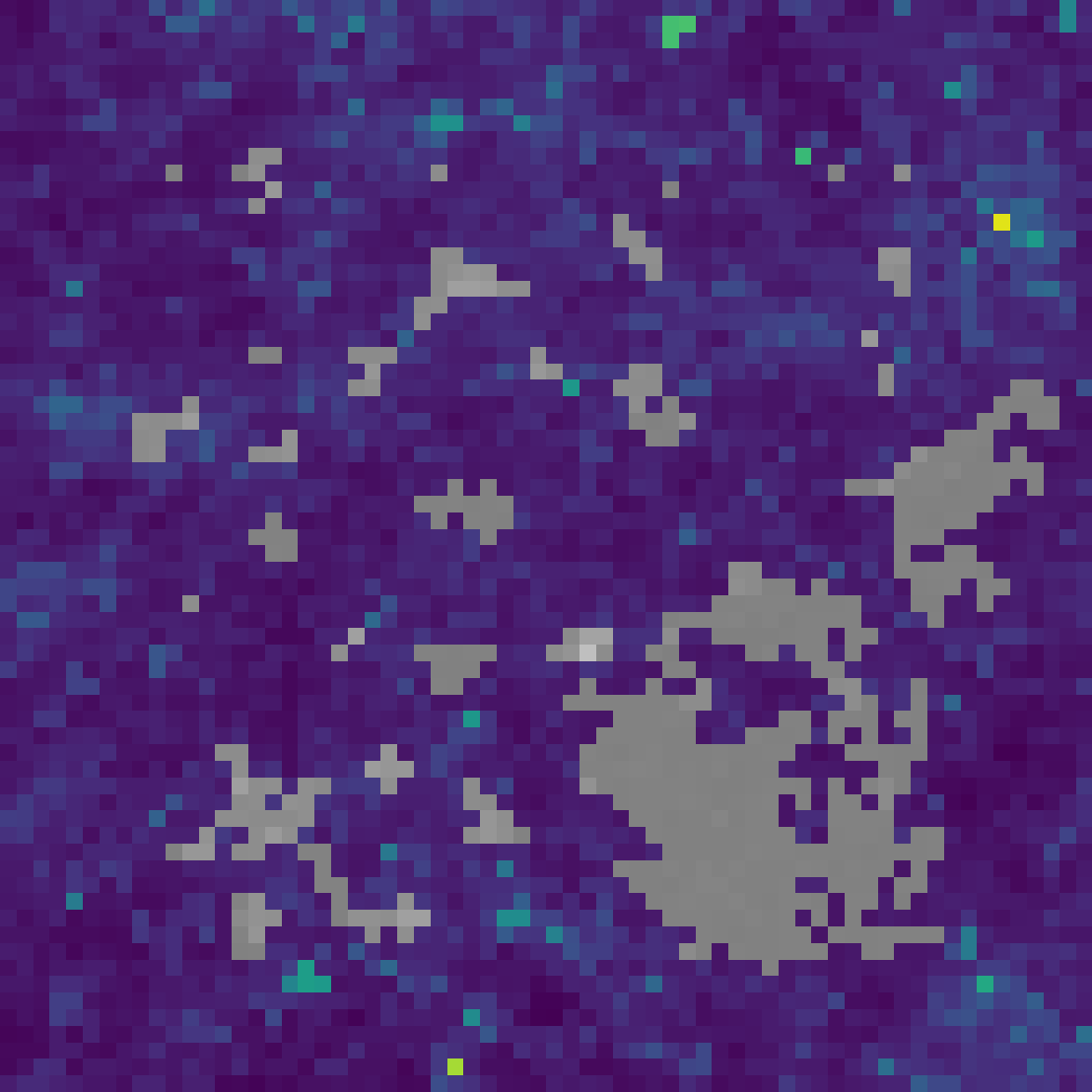
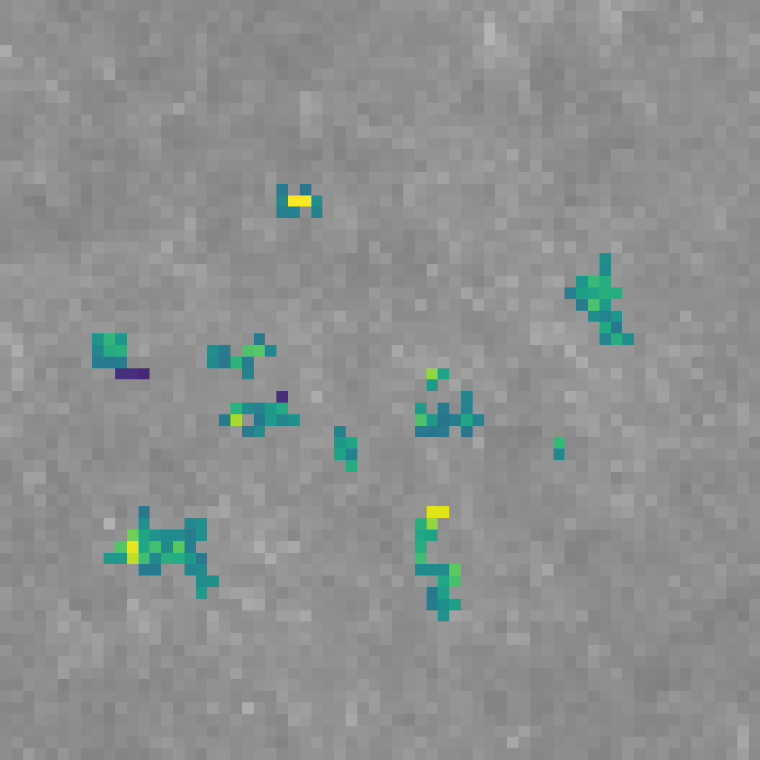
We first find that voids are used more in prediction than clusters in general. This is consistent with previous work that voids are the most important feature in prediction.

Also, voids have especially higher weights for predicting $\Omega_m$ than $\sigma_8$. Clusters, especially high-significance ones, have higher weights for predicting $\sigma_8$.

We can see the distribution of weights in the following histograms:

The first histogram shows that voids have more high weights in the 0.90-1.00 bin for predicting $\Omega_m$. Also, clusters have more low weights in the 0~0.1 bin for predicting $\sigma_8$ as in the second histogram.

Conclusion

In this blog post, we show that group attributions can overcome a fundamental barrier for feature attributions in satisfying faithfulness perturbation tests. Our Sum-of-Parts models generate groups that are semantically meaningful to cosmologists and revealed new properties in cosmological structures such as voids and clusters.

For more details in thoeretical proofs and quantitative experiments, see our paper and code.

Citation

@misc{you2023sumofparts, title={Sum-of-Parts Models: Faithful Attributions for Groups of Features}, author={Weiqiu You and Helen Qu and Marco Gatti and Bhuvnesh Jain and Eric Wong}, year={2023}, eprint={2310.16316}, archivePrefix={arXiv}, primaryClass={cs.LG} }