

Explanation methods for machine learning models tend to not provide any formal guarantees and may not reflect the underlying decision-making process. In this post, we analyze stability as a property for reliable feature attribution methods. We show that relaxed variants of stability are guaranteed if the model is sufficiently Lipschitz smooth to the masking of features. To achieve such a model, we develop a smoothing method called Multiplicative Smoothing (MuS) and demonstrate its theoretical and practical effectiveness.
Modern machine learning models are incredibly powerful at challenging prediction tasks but notoriously black-box in their decision-making. One can therefore achieve impressive performance without fully understanding why. In domains like healthcare, finance, and law, it is not enough that the model is accurate — the model’s reasoning process must also be well-justified and explainable. In order to fully wield the power of such models while ensuring reliability and trust, a user needs accurate and insightful explanations of model behavior.
At its core, explanations of model behavior aim to accurately and succinctly describe why a decision was made, often with human comprehension as the objective. However, what constitutes the form and content of a good explanation is highly context-dependent. A good explanation varies by problem domain (e.g. medical imaging vs. chatbots), the objective function (e.g. classification vs. regression), and the intended audience (e.g. beginners vs. experts). All of these are critical factors to consider when engineering for comprehension. In this post we will focus on a popular family of explanation methods known as feature attributions and study the notion of stability as a formal guarantee.
For surveys on explanation methods in explainable AI (XAI) we refer to Burkart et al. and Nauta et al..
Explanations with Feature Attributions
Feature attribution methods aim to identify the input features (e.g. pixels) most important to the prediction. Given a model and input, a feature attribution method assigns each input feature a score of its importance to the model output. Well known feature attribution methods include: gradient saliency-based (CNN models, Grad-CAM, SmoothGrad), surrogate model-based (LIME, SHAP), axiomatic approaches (Integrated Gradients, SHAP), and many others .
In this post we focus on binary-valued feature attributions, wherein the attribution scores denote the selection (\(1\) values) or exclusion (\(0\) values) of features for the final explanation.

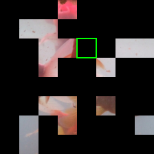
Full image $x$

Explanation $\alpha$
That is, given a model \(f\) and input \(x\) that yields prediction \(y = f(x)\), a feature attribution method \(\varphi\) yields a binary vector \(\alpha = \varphi(x)\) where \(\alpha_i = 1\) if feature \(x_i\) is important for \(y\).
Although many feature attribution methods exist, it is unclear whether they serve as good explanations. In fact, there are surprisingly few papers about the formal mathematical properties of feature attributions as relevant to explanations. However, this gives us considerable freedom when studying such explanations, and we therefore begin with broader considerations about what makes a good explanation. To effectively use any explanation, the user should at minimum consider the following two questions:
- Q1. What is the appropriate metric of quality for evaluating the explanation?
- Q2. Does the explanation behave as expected with respect to this quality metric?
Q1 concerns which inquiry this explanation is intended to resolve. In our context, binary feature attributions aim to answer: “which features are evidence of the predicted class?”, and any metric must appropriately evaluate for this. Q2 is based on the observation that one typically desires an explanation to be “reasonable”. A reasonable explanation promotes confidence as it allows one to “explain the explanation” if necessary.
Q1: Quality Metric for Explanations
We measure the quality of an explanation \(\alpha\) with the original model \(f\). In particular, we evaluate the behavior of \(f(x \odot \alpha)\), where \(\odot\) is the element-wise vector multiplication.
Full image $x$
Explanation $\alpha$

Masked $x \odot \alpha$
Because \(\alpha\) is a binary mask, this form of evaluation can be interpreted as selectively revealing features to the model. This approach is common in domains like computer vision, and indeed modern neural architectures like Vision Transformers can accurately classify even heavily masked images. In particular, it is desirable that an explanation \(\alpha\) can induce the original class, and we formalize this as the notion of consistency.
Definition. (Consistency) An explanation \(\alpha = \varphi(x)\) is consistent if \(f(x) \cong f(x \odot \alpha)\).
Here \(\cong\) means that two model outputs \(y, y'\) indicate the same class. Specifically, we consider classifier models \(f : \mathbb{R}^n \to [0,1]^m\), where the output \(y = f(x)\) is a vector in \([0,1]^m\) whose coordinates denote the confidence scores for the \(m\) classes. Two model outputs therefore satisfy \(y \cong y'\) when they are most confident on the same class.
Q2: Stability as an Expected Behavior
We next consider how an explanation should behave with respect to the above quality metric. Principally, a good explanation \(\alpha = \varphi(x)\) should be strongly confident in its claims, and we express this in two properties. First, the explanation should be consistent, as introduced above in Q1. Second, the explanation should be stable: \(\alpha\) should contain enough salient features, such that including any more features does not alter the induced class.
We present stability as a desirable property because it allows for greater predictability when manipulating explanations. However, many feature attribution methods are not stable! An example of this is shown in the following.
$f(x \odot \alpha) = $ Goldfish
$f(x \odot \alpha') = $ Axolotl
A lack of stability is undesirable, since revealing more of the image should intuitively yield stronger evidence towards the overall prediction. Without stability, slightly modifying an explanation may induce a very different class, which suggests that \(\alpha\) is merely a plausible explanation rather than a convincing explanation. This may undermine user confidence, as a non-stable \(\alpha\) indicates a deficiency of salient features. We summarize these ideas below:
Stability Principle: once the explanatory features are selected, including more features should not induce a different class.
Our work studies stability as a property for reliable feature attributions. We introduce a smoothing method, MuS, that can provide stability guarantees on top of any existing model and feature attribution method.
Stability Properties and Our Approach
In this section we formalize the aforementioned notion of stability and present a high-level description of our approach. First, our definition of stability is defined as follows.
Definition. (Stability) An explanation \(\alpha = \varphi(x)\) is stable if \(f(x \odot \alpha') \cong f(x \odot \alpha)\) for all \(\alpha' \succeq \alpha\).
For two binary vectors we write \(\alpha' \succeq \alpha\) to mean that \(\alpha'\) supersets the selected features of \(\alpha\). That is, \(\alpha' \succeq \alpha\) if and only if each \(\alpha_i ' \geq \alpha_i\). This definition of stability means that augmenting \(\alpha\) with additional features will not significantly change the confidence scores: \(\alpha\) already contains enough salient features to be a convincing explanation. However, it is a challenge to efficiently enforce stability in practice. This is because stability is defined as all \(\alpha' \succeq \alpha\), of which there are exponentially many.
The Plan
In order to extract useful guarantees from the pits of computational intractability, we take the following approach:
- We observe that if the model \(f\) is Lipschitz smooth to the masking of features, one can provably guarantee variants of stability, in particular incremental stability.
- However, many existing and popular models do not have useful Lipschitz smoothness properties by construction. We therefore introduce a smoothing method, MuS, that can provably impose the sufficient Lipschitz smoothness on any model.
- One can then extract guarantees like incremental stability on with any feature attribution method and MuS-smoothed model.
Our stability guarantees are an important result, since, to our knowledge, stability-like guarantees such as this did not previously exist for feature attributions.
Lipschitz Smoothness for Incremental Stability
Fundamentally, Lipschitz smoothness aims to measure the change of a function in response to input perturbations. To quantify perturbations over explanations, we introduce a metric of dissimilarity that counts the differences between binary vectors:
\[\Delta (\alpha, \alpha') = \# \{i : \alpha_i \neq \alpha_i '\}\]In the context of masking inputs, Lipschitz smoothness measures the difference between \(f(x \odot \alpha)\) and \(f(x \odot \alpha')\) as a function of \(\Delta (\alpha, \alpha')\). Given a scalar \(\lambda > 0\), we say that \(f\) is \(\lambda\)-Lipschitz to the masking of features if
\[\mathsf{outputDiff}(f(x \odot \alpha), f(x \odot \alpha')) \leq \lambda \Delta (\alpha, \alpha')\]where \(\mathsf{outputDiff}\) is a metric on the classifier outputs that we detail in our paper. This Lipschitz smoothness means that the change in confidence scores from \(f(x \odot \alpha)\) to \(f(x \odot \alpha')\) is bounded by \(\lambda \Delta (\alpha, \alpha')\). Under this condition: a sufficiently small \(\lambda \Delta (\alpha, \alpha')\) can provably guarantee that \(f(x \odot \alpha) \cong f(x \odot \alpha')\). Observe that a smaller \(\lambda\) is generally desirable, as it allows one to tolerate larger deviations between \(\alpha\) and \(\alpha'\).
Incremental Stability
Lipschitz smoothness gives us the theoretical tooling to examine variants of stability for \(\alpha'\) close to \(\alpha\). In this post we consider incremental stability as one such variant, and consider others in our paper.
Definition. (Incremental Stability) An explanation \(\alpha = \varphi(x)\) is incrementally stable with radius \(r\) if \(f(x \odot \alpha') \cong f(x \odot \alpha)\) for all \(\alpha' \succeq \alpha\) where \(\Delta(\alpha, \alpha') \leq r\).
The radius \(r\) is a conservative theoretical bound on the allowable change to \(\alpha\). A radius of \(r\) means that, provably, up to \(r\) features may be added to \(\alpha\) without altering its induced class. Different inputs may have different radii, and note that we need \(r \geq 1\) to have a non-trivial incremental stability guarantee. Quantifying this radius in relation to the Lipschitz smoothness of \(f\) is one of our main results (Step 3 of The Plan), sketched below.
Theorem Sketch. (Radius of Incremental Stability) Suppose that \(f\) is \(\lambda\)-Lipschitz to the masking of features, then an explanation \(\alpha = \varphi(x)\) is incrementally stable with radius \(r = \mathsf{confidenceGap}(f(x \odot \alpha)) / (2 \lambda)\).
The \(\mathsf{confidenceGap}\) function computes the difference between the first and second highest confidence classes. A greater confidence gap indicates that \(f\) is more confident about its prediction, and that the second-best choice does not even come close.
However, the above criteria are contingent on the classifier \(f\) satisfying the relevant Lipschitz smoothness, which does not hold for most existing and popular classifiers! This thereby motivates using a smoothing method, like MuS, to impose such smoothness properties.
MuS for Lipschitz Smoothness
The goal of smoothing is to transform a base classifier \(h : \mathbb{R}^n \to [0,1]^m\) into a smoothed classifier \(f : \mathbb{R}^n \to [0,1]^m\), such that \(f\) is \(\lambda\)-Lipschitz with respect to the masking of features. This base classifier may be any classifier, e.g. ResNet, Vision Transformer, etc. Our key insight is that randomly dropping features from the input attains the desired smoothness, which we will simulate by sampling \(N\) binary masks \(s^{(1)}, \ldots, s^{(N)} \sim \mathcal{D}\). Many choices of \(\mathcal{D}\) in fact work, but one may intuit it as the \(n\)-dimensional coordinate-wise iid \(\lambda\)-parameter Bernoulli distribution \(\mathcal{B}^n(\lambda)\).
Given input \(x\) and base classifier \(h\), the evaluation of \(f(x)\) may be understood in three stages.
- (Stage 1) Sample binary masks \(s^{(1)}, \ldots, s^{(N)} \sim \mathcal{D}\).
- (Stage 2) Generate masked inputs \(x \odot s^{(1)}, \ldots, x \odot s^{(N)}\).
- (Stage 3) Average over \(h(x \odot s^{(1)}), \ldots, h(x \odot s^{(N)})\). This average is the value of \(f(x)\).
In expectation, this \(f\) is \(\lambda\)-Lipschitz with respect to the masking of features. We remark that \(\lambda\) is fixed before smoothing, and that this three-stage smoothing is applied for any input: even explanation-masked inputs like \(x = x' \odot \alpha\).
Although it is simple to view \(\mathcal{D}\) as \(\mathcal{B}^n (\lambda)\), there are multiple valid choices for \(\mathcal{D}\). In particular, it suffices that each coordinate of \(s \sim \mathcal{D}\) is marginally Bernoulli: that is, each \(s_i \sim \mathcal{B}(\lambda)\). The distribution \(\mathcal{B}^n (\lambda)\) satisfies this marginality condition, but so will others. We now present our main smoothing result.
Theorem Sketch. (MuS) Let \(s \sim \mathcal{D}\) be any random binary vector where each coordinate is marginally \(s_i \sim \mathcal{B}(\lambda)\). Consider any \(h\) and define \(f(x) = \underset{s \sim \mathcal{D}}{\mathbb{E}}\, h(x \odot s)\), then \(f\) is \(\lambda\)-Lipschitz to the masking of features.
This generic form of \(\mathcal{D}\) has strong implications for efficiently evaluating \(f\): if \(\mathcal{D}\) were coordinate-wise independent (e.g. \(\mathcal{B}^n(\lambda)\)), then one needs \(N = 2^n\) deterministic samples of \(s \sim \mathcal{D}\) to exactly compute \(f(x)\), which may be expensive. We further discuss in our paper how one can construct \(\mathcal{D}\) with statistical dependence to allow for efficient evaluations of \(f\) in \(N \ll 2^n\) samples.
Empirical Evaluations
To evaluate the practicality of MuS, we ask the following: can MuS obtain non-trivial guarantees in practice? We show that this is indeed the case!
Experimental Finding: MuS can achieve non-trivial guarantees on off-the-shelf feature attribution methods and classification models.
Moreover, the stability guarantees are obtained with only a light penalty to accuracy. These results of guarantees are significant, because not only are the formal properties of feature attributions not well known, there are in fact results about their limitations.
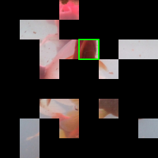
In this post we present experiments that test whether one can yield non-trivial guarantees from a popular feature attribution method, SHAP. We select the top-25% scoring features of SHAP to be our explanation method \(\varphi\), we take our classifier \(f\) to be Vision Transformer, and we sample \(N = 2000\) image inputs \(x\) from ImageNet1K. We are interested in the different qualities of guarantees obtained as one varies the smoothing parameter \(\lambda\). Below we plot the fraction of images that satisfy incremental stability (and consistency) up to some radius, where we express this radius as a fraction \(r/n\) of the total features.
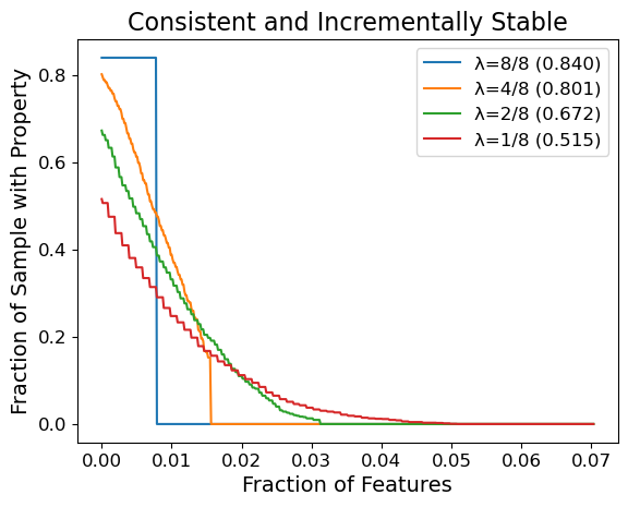
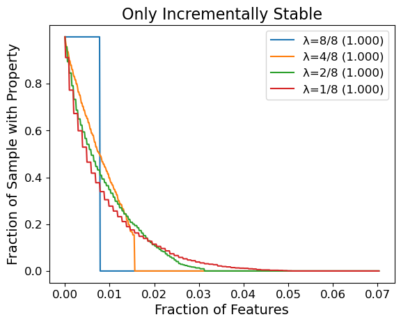
For instance with \(\lambda = 1/8\), about \(20\%\) of the samples achieve both consistency and incremental stability with radius \(\geq 1\%\) of the image (\((3 \times 224 \times 224) \times 0.01 \approx 1500\) features). If we omit the consistency requirement, then even more images achieve the same radius. To our knowledge, these are important results: prior to our work there were no formal guarantees for stability-like properties on general feature attribution methods for generic models. In addition, SHAP is not explicitly designed for stability, so it is significant that even a simple modification like top-25% selection can yield non-trivial guarantees. It is future work to investigate feature attribution methods that are better suited to maximizing such guarantees.
We remark there is an upper-bound on the radius of stability MuS can guarantee: we will always have a radius of \(r \leq 1 / (2 \lambda)\), which explains why curves for the same value of \(\lambda\) have the same zero-points. This upper-bound is because our results for smoothing requires that the classifier \(f\) be bounded, and we pick a range of \([0,1]^m\) without loss of generality. To work around this theoretical limitation, we present in our paper some parametrization strategies that allow for greater radii of stability.
Finally, we refer to our paper for a comprehensive suite of experiments that evaluate the effectiveness of MuS across vision and language models along with different feature attribution methods.
Conclusion
In this post we presented stability guarantees as a formal property for feature attribution methods: a selection of features is stable if the additional inclusion of other features do not alter its induced class. We showed that if the classifier is Lipschitz with respect to the masking of features, then one can guarantee incremental stability. To achieve this Lipschitz smoothness we developed a smoothing method called Multiplicative Smoothing (MuS) and analyzed its theoretical properties. We showed that MuS achieves non-trivial stability guarantees on existing feature attribution methods and classifier models.
Citation
@misc{xue2023stability,
author = {Anton Xue and Rajeev Alur and Eric Wong},
title = {Stability Guarantees for Feature Attributions with Multiplicative Smoothing},
year = {2023},
eprint = {2307.05902},
archivePrefix = {arXiv},
primaryClass = {cs.LG}
}