
This post introduces CTSketch, an algorithm for learning tasks expressed as the composition of neural networks followed by a symbolic program (neurosymbolic learning). CTSketch decomposes the symbolic program using tensor sketches summarizing the input-output pairs of each sub-program and performs fast inference via efficient tensor operations. CTSketch pushes the frontier of neurosymbolic learning, scaling to tasks involving over one thousand inputs, which has never been done before.
Many learning problems benefit from combining neural and symbolic components to improve accuracy and interpretability. In our previous blog post, we introduced a natural decomposition of the scene recognition problem, which involves a neural object detector and a program that prompts GPT-4 to classify the scene based on the object predictions.
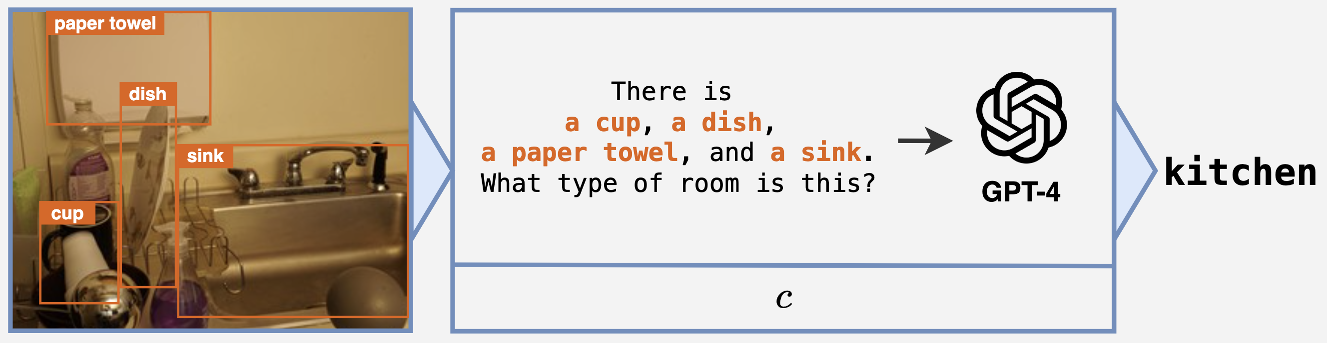
This learning paradigm, called neurosymbolic learning, targets the composition of a neural network $M_\theta$ followed by a program $c$, and the goal is to train $M_\theta$ with end-to-end labels of the composite.
White- and Black-Box Neurosymbolic Programs
In the previous post, we also categorized neurosymbolic methods into white- and black-boxes based on their accessibility to the internals of programs.
White-box neurosymbolic programs usually take the form of differentiable logic programs. While white-box programs can be easier to learn with, many logic-program-based programs are incompatible with Python programs (neuroPython) and programs that call GPT (neuroGPT), which are useful for leaf classification and scene recognition tasks.
On the other hand, black-box neurosymbolic programs, also known as neural programs, target a more challenging setting where programs can be written in any language and involve API calls. This includes neural approximation methods that train surrogate neural models of programs. Despite scaling to tasks with combinatorial difficulty, they struggle to learn programs involving complex reasoning, like Sudoku solving.
Moreover, prior work on white- and black-box learning has not been able to scale to tasks with a large number of inputs, like one thousand inputs. Such limitations motivate a scalable solution that combines the strengths of both approaches.
CTSketch: Key Insights
We introduce CTSketch, a novel learning algorithm that uses two techniques to scale: decompose the program into multiple sub-programs and summarize each sub-program with a sketched tensor.
Program Decomposition
While CTSketch supports black-box programs, its scalability benefits from program decomposition. The complexity of neurosymbolic inference grows with the input space of the program, so decomposing into sub-programs, each with a smaller number of inputs and exponentially smaller input space, makes the overall computation more affordable.
CTSketch works with any manually specified tree structure of sub-programs, where the first layer of programs corresponds to the leaves and the last sub-program, which predicts the final output, represents the root. The sub-programs are evaluated sequentially layer-by-layer, and the outputs from sub-programs further from the root are fed into sub-programs closer to the root.
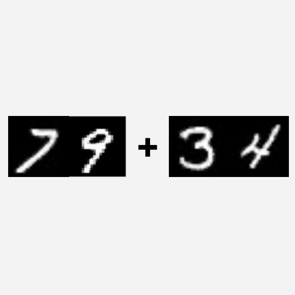
Click on the thumbnails to see different examples of program decomposition. The decomposition does not need to form a perfect tree, and programs with bounded loops like add-2 can be decomposed into repeated layers.
-
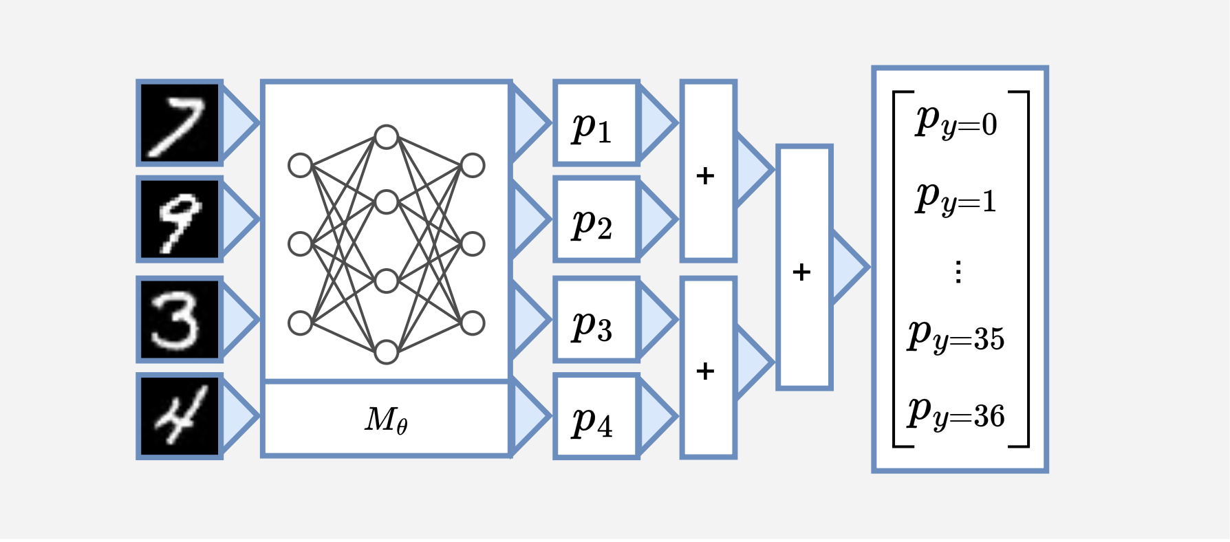
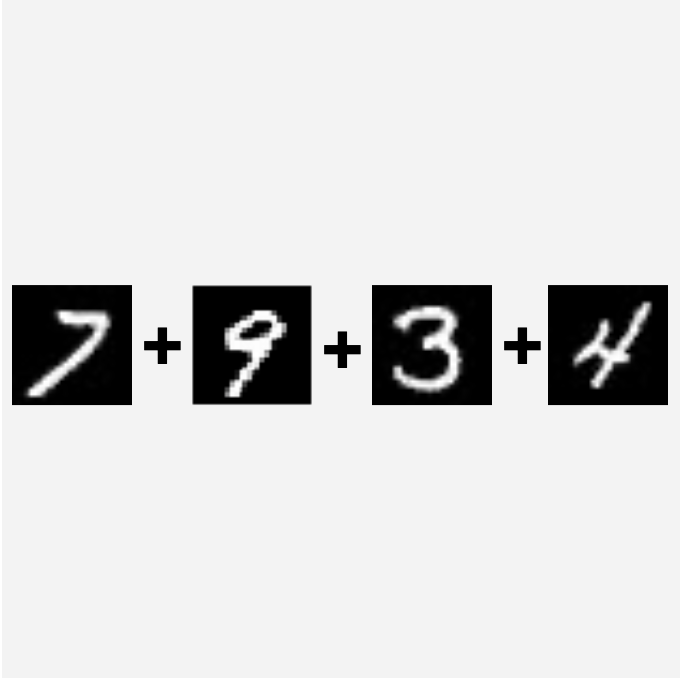
Program decomposition for MNIST sum of 4 digits (Sum-4). -
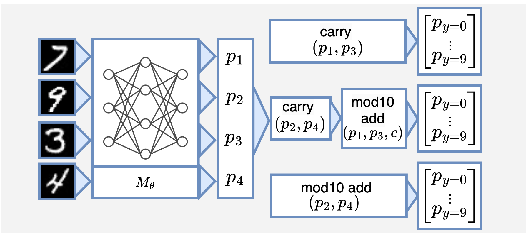
Program decomposition for MNIST addition of two 2-digit numbers (Add-2). -
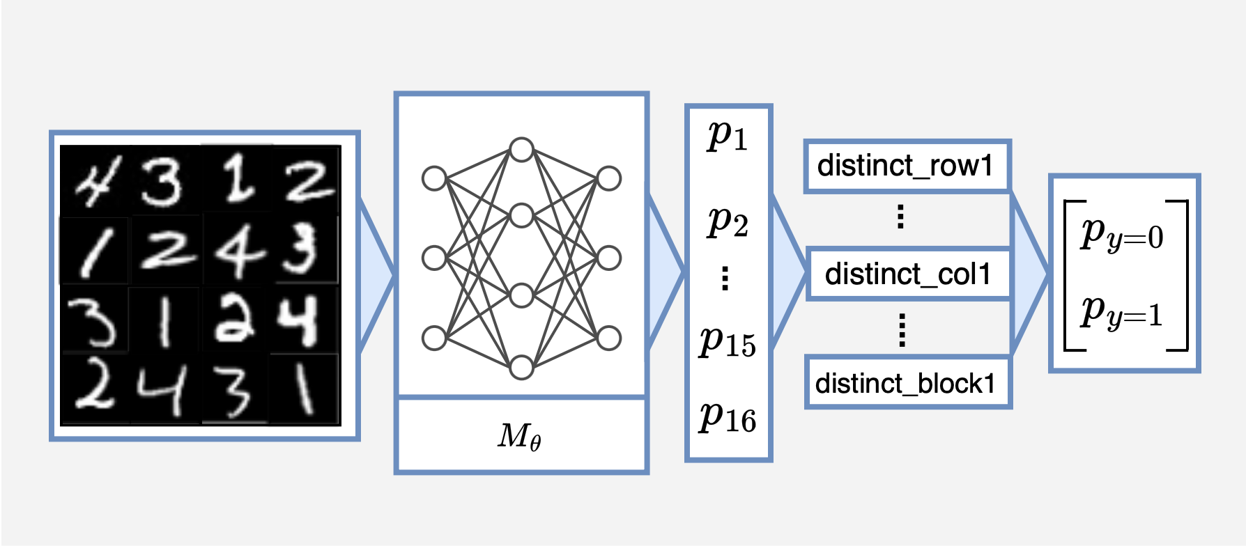
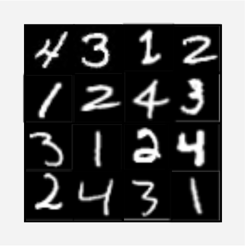
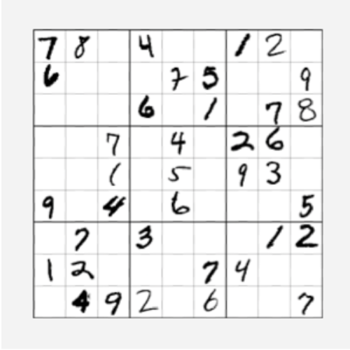
Program decomposition for checking whether it is a valid Sudoku board. -
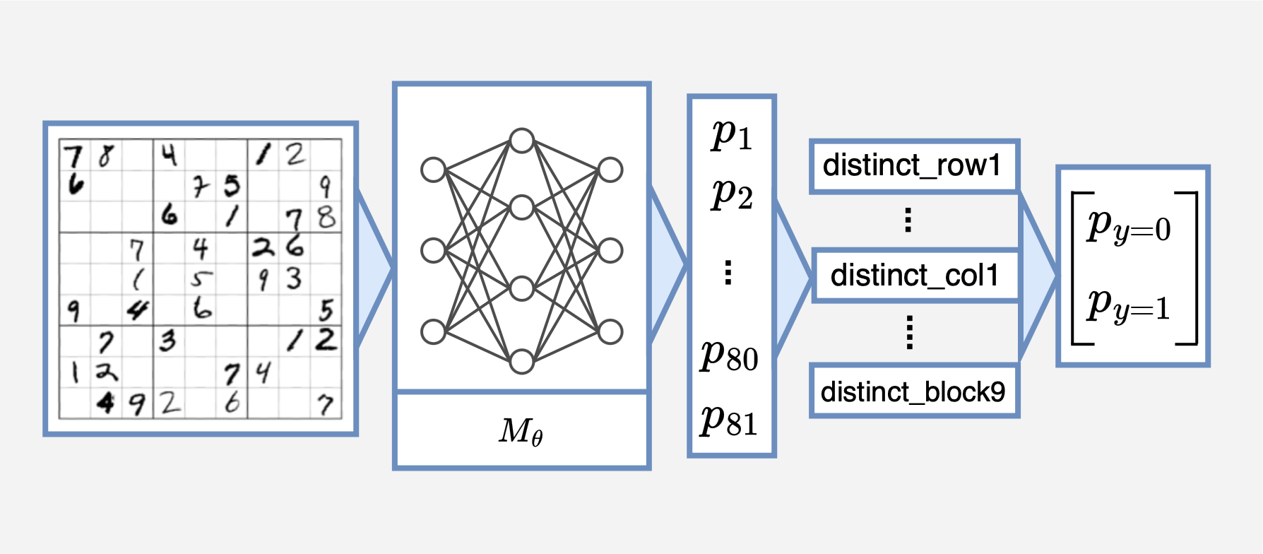
Program decomposition for solving Sudoku.
As illustrated in the figure, we can decompose the sum-4 task into a hierarchy of sum-2 operations.
The new structure consists of a $+$ function (sub-program $c_1$) that adds two numbers between 0-9 and another $+$ function ($c_2$) that adds two numbers between 0-18. The final output is computed as $c_2(c_1(p_1, p_2), c_1(p_3, p_4))$, where $p_1, \dots, p_4$ are probability distributions output by the neural network.
Summary Tensor
We summarize each sub-program using a tensor, where each dimension of the tensor corresponds to each program input. For a sub-program $c_i$ that takes $d$ inputs from a finite domain, its summary tensor $\phi_i$ is a $d$-dimensional tensor that satisfies $\phi_i[j_1, \dots, j_d] = c_i(j_1, \dots, j_d)$.
The summary tensors preserve the program semantics in terms of input-output relationships. Furthermore, they enable efficient computation of the program output, only using simple tensor operations over the tensor summaries and the input probabilities.
The sum-4 task uses two different tensors $\phi_1: \mathbb{R}^{10 \times 10}$ and $\phi_2: \mathbb{R}^{19 \times 19}$, where for both cases $\phi_i[a, b] = a + b$.
CTSketch: Algorithm
Prior to training, CTSketch goes through two steps: tensor initialization and sketching. CTSketch prepares the summary tensor beforehand to make the training pipeline end-to-end differentiable without any calls to the program.
Tensor Initialization and Sketching
CTSketch initializes each summary tensor $\phi_i$ by sampling a subset or enumerating all input combinations. We query the program with each input and fill in the corresponding entry with the output.
To further improve time and space efficiency, we reduce the size of the tensor summaries using low-rank tensor decomposition methods. These techniques find low-rank tensors, called sketches, that reconstruct the original tensor with low error guarantees and exponentially less memory.
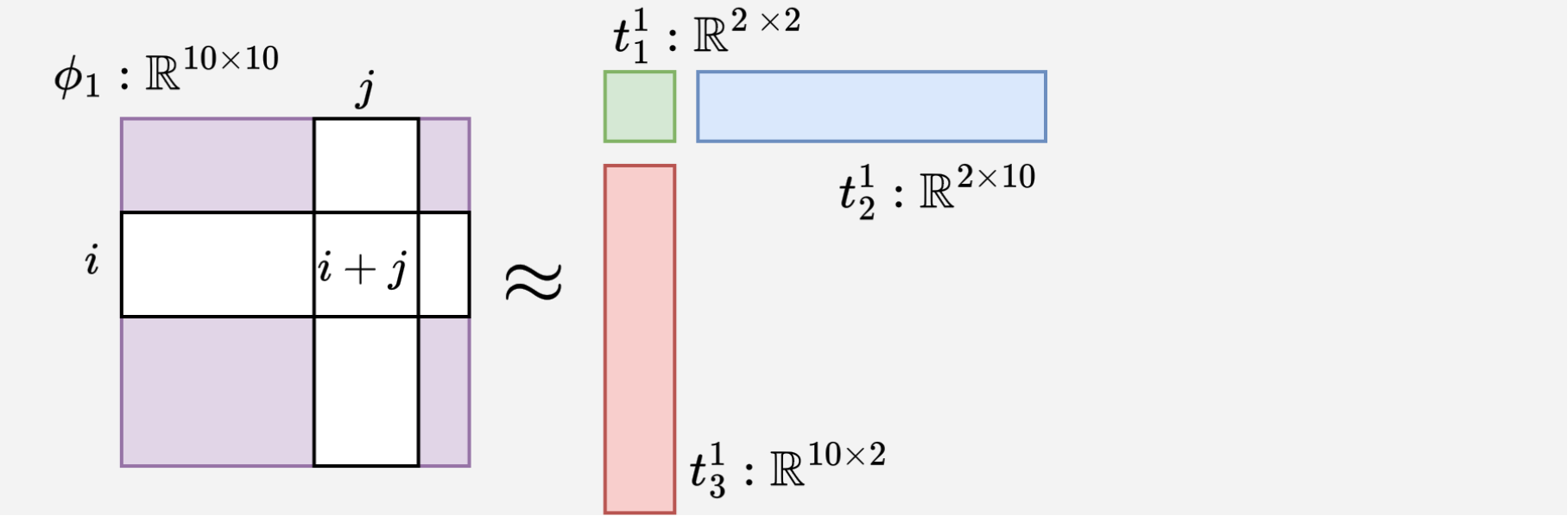
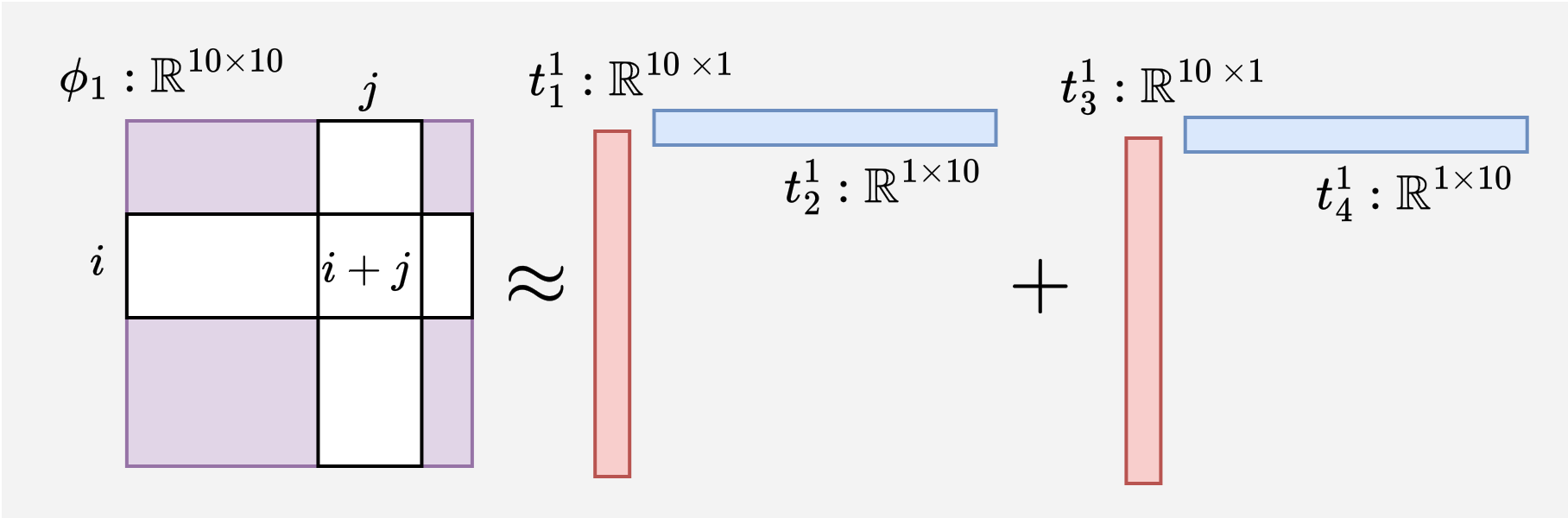
See the rank-2 sketches produced by different decomposition methods for the $\phi_1$ in the sum-4 example.
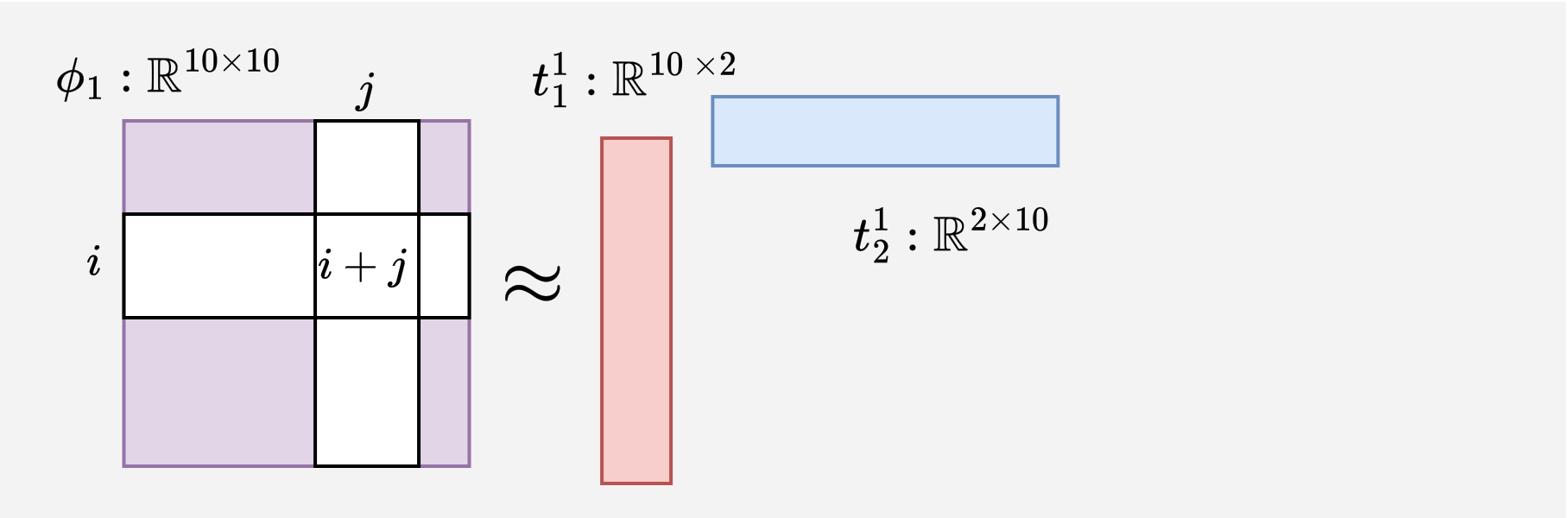
For sum-4, we apply TT-SVD with the decomposition rank configured to 2 and obtain two sketches $t_1^1 : \mathbb{R}^{10 \times 2}$ and $t_2^1 : \mathbb{R}^{2 \times 10}$ for $\phi_1$.
Training
The training pipeline for sum-4 can be summarized as:
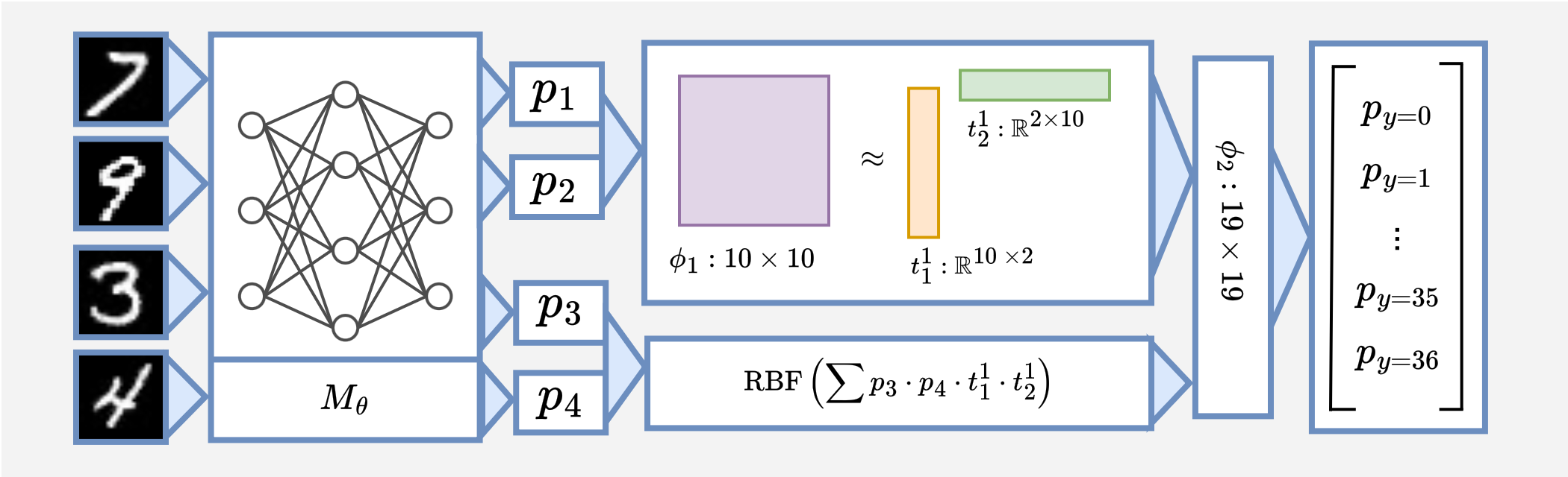
Inference proceeds through program layers and estimates the expected output for each sub-program. In the case of the first sum-2 sub-program ($\phi_1 \approx t_1^1 \times t_2^1$) and probability distributions $p_1$ and $p_2$, we compute the expected output without reconstructing the full program tensor as:
\[v = \sum_a^{10} \sum_b^{10} \sum_x^2 p_1[a] p_2[b] t_1^1[a, x] t_2^1[x, b] \\ = \sum_x^2 \left(\sum_a^{10} p_1[a] t_1^1[a, x]\right) \left(\sum_b^{10} p_2[b]t_2^1[x, b]\right) \\ = (p_1^{\top} t_1^1) \cdot (t_2^1 p_2)\]Then, we apply RBF kernel and $L_1$ normalization to transform the value $v$ into a probability distribution. For each output value $j$, we use the following formula:
\[p[j] = \frac{\text{RBF}(v, j)}{\sum_{k=0}^{18}\text{RBF}(v, k)} = \frac{\text{exp} \left( -\frac{1}{2\sigma^2}||v - j||_2 \right)}{\sum_{k=0}^{18} \text{exp} \left( -\frac{1}{2\sigma^2}||v - j||_2 \right)}\]The resulting distributions are passed on to the second layer as inputs, where this process repeats and produces the final output.
The final output can be directly compared with the ground truth output without undergoing such transformation; hence, the final output space can be infinite, such as floating-point numbers.
Test and Inference
Using sketches for inference is efficient but potentially biased due to the approximation error. After training, we call the symbolic program with the argmax inputs instead.
Evaluation
To answer the research question Can CTSketch solve tasks unsolvable by existing methods?, we consider sum-1024, a task with orders of magnitude larger input size than previously studied.
| sum-4 | sum-16 | sum-64 | sum-256 | sum-1024 | |
|---|---|---|---|---|---|
| Scallop | 88.90 | 8.43 | TO | TO | TO |
| DSL | 94.13 | 2.19 | TO | TO | TO |
| IndeCateR | 92.55 | 83.01 | 44.43 | 0.51 | 0.60 |
| ISED | 90.79 | 73.50 | 1.50 | 0.64 | ERR |
| A-NeSI | 93.53 | 17.14 | 10.39 | 0.93 | 1.21 |
| CTSketch | 92.17 | 83.84 | 47.14 | 7.76 | 2.73 |
The baseline methods fail to learn sum-256, whereas CTSketch attains 93.69% per-digit accuracy on sum-1024. In contrast, it stays at 17.92% for the next-best performer, A-NeSI. The baselines struggle due to the weak learning signal from supervising only the final output.
Check our paper for experiments on standard neurosymbolic benchmarks, including Sudoku solving, scene recognition using GPT, and HWF with infinite output space. The results demonstrate that CTSketch is competitive with SOTA frameworks while converging faster.
Limitations and Future Work
The primary limitation of CTSketch lies in requiring manual decomposition of the symbolic component to scale, motivating future work on automating the decomposition using program synthesis techniques.
Another interesting future direction is exploring different tensor sketching methods and the trade-offs they provide. For example, a streaming algorithm would significantly reduce memory requirements with a small time overhead while initializing tensor sketches.
Conclusion
We proposed CTSketch, a framework that uses decomposed programs to scale neurosymbolic learning. CTSketch uses sketched tensors representing the summary of each sub-program to efficiently approximate the output distribution of the symbolic component using simple tensor operations. We demonstrate that CTSketch pushes the frontier of neurosymbolic learning, solving significantly larger problems than prior works could solve while remaining competitive with existing techniques on standard neurosymbolic learning benchmarks.
For more details about our method and experiments, see our paper and code.
Citation
@article{choi2025CTSketch,
  title={CTSketch: Compositional Tensor Sketching for Scalable Neurosymbolic Learning},
  author={Choi, Seewon and Solko-Breslin, Alaia and Alur, Rajeev and Wong, Eric},
  journal={arXiv preprint arXiv:2503.24123},
  year={2025}
}